Chemistry machine learning for drug discovery with DeepChem

This example uses machine learning to predict the lipophilicity of compounds.

Lipophilicity measures how well a compound dissolves in non-polar media such as fats and lipids. So it’s important for drugs that are delivered orally (for example, via a pill) because the active ingredient needs to be absorbed into the lipids of biological membranes.

Open this notebook in Google Colab

%%capture
!pip install --pre deepchem[tensorflow]

#For mol_frame
%%capture
!pip install git+https://github.com/apahl/mol_frame

from mol_frame import mol_frame as mf
import os, holoviews as hv
os.environ['HV_DOC_HTML'] = 'true'

import deepchem as dc
import seaborn
import pandas as pd
import matplotlib.pyplot as plt

DeepChem is a free and open-source Python package for deep learning for chemistry and other sciences. DeepChem has a lipophilicity data set contains measured logD values for 4200 compounds.

As usual for machine learning (ML), we split the data set into training and test data. We train the ML model on the train data, then apply it to the test data and check how well the model predicts the lipophilicity of compounds that the model hasn’t processed before.

For this data set, we split by scaffold the 4200 compounds based on the Bemis-Murcko scaffold representation. Such splitting groups molecules based on their scaffolds (core structure) to prevent train and test from having very similar molecules, which could lead to the model appearing to perform well on the test set, but then performing poorly on less-similar molecules in production.

tasks, datasets, transformers = dc.molnet.load_lipo(featurizer='GraphConv', splitter='Scaffold')
train_dataset, valid_dataset, test_dataset = datasets

The number of compounds in the train, validate, and test sets is:

splits = (train_dataset.X.shape[0], valid_dataset.X.shape[0], test_dataset.X.shape[0])
splits

(3360, 420, 420)

Which represents an 80:10:10 train:validate:test split:

[split / sum(splits) for split in splits]

[0.8, 0.1, 0.1]

Next, we build a model using DeepChem’s graph convolutional network. We use the dropout technique to avoid overfitting.

model = dc.models.GraphConvModel(n_tasks=1, mode='regression', dropout=0.2)

Then we train the model on the train dataset.

# Note that training with 200 epochs takes around 8 minutes on Google Colab.
# If you are debugging or just running a proof of concept, you may want to set nb_epoch=10 to speed execution.
%%capture
model.fit(train_dataset, nb_epoch=200);

To check how well the model fits the train and test data, we examine the Pearson correlation coefficient score. Its value can range from -1 to 1, where positive values indicate postive correlation, zero indicates no correlation, and negative values indicate negative correlation. The magnitude of the value indicates the strength of the correlation: less than 0.3 is weak, 0.3-0.5 is moderate, and 0.5-1 is strong.

metric = dc.metrics.Metric(dc.metrics.pearson_r2_score)
print("Training set score:", model.evaluate(train_dataset, [metric], transformers))
print("Test set score:", model.evaluate(test_dataset, [metric], transformers))

Training set score: {'pearson_r2_score': 0.8866760139249386}
Test set score: {'pearson_r2_score': 0.5358381141161308}

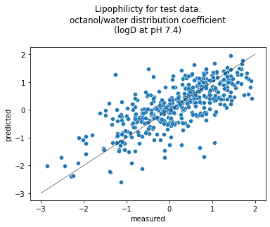
The Pearson correlation coefficient score is worse for the test data than for the train data. This is expected because the test data is new to the model. Nevertheless, the magnitude being greater than 0.5 indicates a strong, positive correlation betwen predicted and measued lipophilicity.

One contributing factor might be that our train set may not have molecules similar enough to those in the test set. Recall that we split by scaffold, so it’s possible that such splitting led to compounds in the test set that have scaffolds significantly different from those in the train set.

Adding compounds to the dataset so that there is less “scaffold distance” (difference in scaffold structure) between groups of compounds might help. To take a simple hypothetical example, if we had a dataset with compounds containing fused rings, with many two-ring compounds and few four-ring compounds, scaffold splitting might put all the two-ring compounds in the train set and all the four-ring compounds in the test set. We expect that would lead to poor predictions on the test set. We would want to augment the dataset by adding compounds containing three fused rings.

To learn more about how well the model works, let’s apply it to the test data and compare the predicted and experimental results.

lipos = model.predict_on_batch(test_dataset.X)

Then we put the measured and model-predicted results into a pandas dataframe for easy processing.

lipo_list = []
expt_lipo_list = []
for molecule, lipo, test_lipo in zip(test_dataset.ids, lipos, test_dataset.y):
    lipo_list += [lipo[0]]
    expt_lipo_list += [test_lipo[0]]
    
compound_id = list(range(len(test_dataset.ids)))
df = pd.DataFrame(list(zip(expt_lipo_list, lipo_list, test_dataset.ids, compound_id)), columns = ["measured", "predicted", "Smiles", "Compound_Id"])
df

	measured	predicted	Smiles	Compound_Id
0	-1.810832	-0.892024	O[C@@H](CNCCCOCCNCCc1cccc(Cl)c1)c2ccc(O)c3NC(=O)Sc23	0
1	0.319651	-0.728260	NC1=NN(CC1)c2cccc(c2)C(F)(F)F	1
2	-0.192325	0.023027	COc1cc(ccc1Cn2ccc3ccc(cc23)C(=O)NCC4CCCC4)C(=O)NS(=O)(=O)c5ccccc5	2
3	0.938978	0.337164	NC(=O)NC(=O)C(Nc1ccc2CCCc2c1)c3ccccc3	3
4	0.856401	0.464554	COc1ccc(cn1)c2ccc3nc(N)sc3c2	4
...	...	...	...	...
415	0.815112	1.280881	COc1cc(ccc1N2CC[C@@H](O)C2)N3N=Nc4cc(sc4C3=O)c5ccc(Cl)cc5	415
416	1.327089	0.092211	CCC(COC(=O)c1cc(OC)c(OC)c(OC)c1)(N(C)C)c2ccccc2	416
417	-0.175810	0.370334	CCCSc1ncccc1C(=O)N2CCCC2c3ccncc3	417
418	0.071921	-0.493196	Oc1ncnc2scc(c3ccsc3)c12	418
419	0.806855	0.264380	OC1(CN2CCC1CC2)C#Cc3ccc(cc3)c4ccccc4	419

420 rows × 4 columns

Now we can use a scatter plot to compare the predicted against measured values. We use the seaborn statistical data visualization package to plot the data. We show the line where the predicted and measured lipophilicity values are equal, in other words the line that all points would lie on if the model made perfect predictions.

seaborn.scatterplot(data=df, x = "measured", y = "predicted").set(title='Lipophilicity for test data:\noctanol/water distribution coefficient\n(logD at pH 7.4)\n');
equal_line_x = [-3, 2]
equal_line_y = equal_line_x
plt.plot(equal_line_x, equal_line_y, color='k', linewidth=0.5);

We can also use mol_frame to make an interactive plot: If you mouse over a marker on the graph, the molecular structure will be displayed! (One interesting thing to note is that molecules which are close together on the plot may have very different molecular structures.) Also, you can pan and zoom the graph, and save it.

Unfortunately, the interactive plot is not working in the blog version of this notebook. Please visit the Google Colab notebook to access the interactive plot.

cpds = mf.MolFrame(df)
cpds = cpds.add_b64()
hv.extension('bokeh')
cpds.scatter("measured", "predicted")

* using Smiles
* add b64:               (  420 |    5)

* using Mol_b64
* add img:               (  420 |    6)

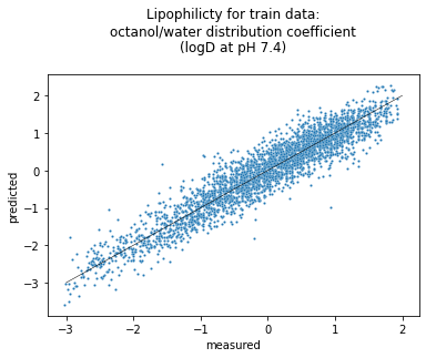
Let’s plot the train data set to visually compare those two sets. We made the markers (points) smaller because there are so many and we don’t want them to overlap with each other so much.

lipos_train = model.predict_on_batch(train_dataset.X)
lipo_list_train = []
expt_lipo_list_train = []
for molecule, lipo, test_lipo in zip(train_dataset.ids, lipos_train, train_dataset.y):
    lipo_list_train += [lipo[0]]
    expt_lipo_list_train += [test_lipo[0]]
df_train = pd.DataFrame(list(zip(expt_lipo_list_train, lipo_list_train)), columns = ["measured", "predicted"])
seaborn.scatterplot(data=df_train, x = "measured", y = "predicted", s=5, palette=["orange"]).set(title='Lipophilicity for train data:\noctanol/water distribution coefficient\n(logD at pH 7.4)\n');
plt.plot(equal_line_x, equal_line_y, color='k', linewidth=0.5);

Unfortunately, mol_frame takes too long to render thousands of molecules so that Google Colab disconnects before it completes. So we’re not showing the interactive plot here. You probably could if you ran this notebook locally.

To overlay the two plots, we’ll first concatenate the data in the two sets (test and train), adding a dataset column to keep track of which set each point came from.

# Remove the columns we added to the test dataframe for mol_frame
try:
  df.drop(columns=["Smiles", "Compound_Id"], inplace=True)
except:
  # Suppress any error if those columns have already been dropped
  pass

concatenated = pd.concat([df.assign(dataset='test'), df_train.assign(dataset='train')])
concatenated

	measured	predicted	dataset
0	-1.810832	-0.892024	test
1	0.319651	-0.728260	test
2	-0.192325	0.023027	test
3	0.938978	0.337164	test
4	0.856401	0.464554	test
...	...	...	...
3355	0.526093	-0.117241	train
3356	-0.027172	-0.238245	train
3357	-1.629163	-1.749196	train
3358	0.633443	0.961528	train
3359	-0.960290	-1.251761	train

3780 rows × 3 columns

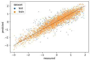
Now we can plot the two datasets on one graph.

seaborn.scatterplot(x='measured', 
                    y='predicted', 
                    data=concatenated,
                    hue='dataset',
                    s=5);
plt.plot(equal_line_x, equal_line_y, color='k', linewidth=0.5);

Some of the test (blue) data points are predicted (on the vertical axis) outliers, reflecting that the model performs poorly for them. We might consider featurizing our data further to let the model predict lipophilicity based on more properties of the compounds. Above, we used the GraphConv featurizer, which represents only the atoms in a molecule. We might try the WeaveFeaturizer which also represents the bonds, though it requires more resources because it stores the relationship between each pair of atoms in a molecule.

This blog post was based on the DeepChem tutorial The Basic Tools of the Deep Life Sciences. Thanks to mol_frame author Axel Pahl for making that package usable from Google Colab.

This post was updated on December 28, 2022 to explain the Pearson correlation coefficient and increase the number of training epochs from 100 to 200.