Refitting Data From Wiener’s Classic Cheminformatics Paper
In a previous post, I revisited Wiener’s paper predicting alkanes’ boiling points using modern cheminformatics tools. This follow-up post refits the data with modern mathematical tools to check how well the literature parameters, and the current parameters optimized here, fit the data.
Wiener and Egloff’s works are impressive for using cheminformatics parameters that model physical data with simple relationships. Let’s double-check how well their models fit the data. Equations reference Wiener’s 1947 Journal of the American Chemical Society article “Structural Determination of Paraffin Boiling Points”.
Egloff modeled boiling point $t_{0}$ for linear alkanes as a function of the number of carbon atoms $n$:
$t_{0} = 745.42 \log(n + 4.4) - 689.4$ (eqn 5)
Wiener modeled boiling point difference ($\Delta t$) for a general alkane compared to its straight-chain isomer as a function of the difference in the polarity number $p$ and the Wiener index (path number) $\omega$:
$\Delta t = \frac{k}{n^{2}}\Delta\omega + b\Delta p$ (eqn 3)
Wiener fit that model to the data to find values $k$ = 98 and b = 5.5:
$\Delta t = \frac{98}{n^{2}}\Delta\omega + 5.5\Delta p$ (eqn 4)
Open this notebook in Google Colab so you can run it without installing anything on your computer
Approach Used in This Blog Post
Rather than redo all the data ingestion and manipulation from my previous post, I exported the dataframes and then imported them here. I then used scipy optimize curve_fit to fit the data.
The key packages this post uses are:
- scipy to fit the data
- Polars to track the information for the molecules in DataFrames
- seaborn and matplotlib to plot the results
- mol_frame to show images of molecules when you mouse over them on a graph
%%capture
%pip install scipy
%pip install numpy
%pip install polars
%pip install black[jupyter]
%pip install seaborn
# For mol_frame
%%capture
%pip install git+https://github.com/apahl/mol_frame

from mol_frame import mol_frame as mf
import os, holoviews as hv

os.environ["HV_DOC_HTML"] = "true"
import numpy as np
import matplotlib.pyplot as plt
from scipy.optimize import curve_fit
import polars as pl
import math
import seaborn
from typing import Callable
from collections.abc import Iterable
from matplotlib.lines import Line2D
Quantifying Goodness of Fit
R-Squared, the coefficient of determination, is a standard metric for checking how good a fit is. A value of 1 indicates a perfect fit.
$R^2 = 1 - \frac{SS_{residuals}}{SS_{total}}$
where $SS$ means sum of squares. The residuals reflect how imperfect the fit is, that is the difference between an actual data point $y_{i}$ and the fit for that data point $f_{i}$:
$residual_{i} = y_{i}-f_{i}$
$SS_{residuals} = \displaystyle\sum_{i}{(y_{i}-f_{i})^2}$
The denominator is proportional to the variance of the data, that is the difference between each data point $y_{i}$ and the mean of all data points $\bar{y}$:
$SS_{total} = \displaystyle\sum_{i}{(y_{i}-\bar{y})^2}$
R-Squared determination is implemented just that way using this function:
def r_squared(f: Callable, xdata: Iterable, ydata: Iterable, popt: Iterable):
    """
    From https://stackoverflow.com/questions/19189362/getting-the-r-squared-value-using-curve-fit
    :returns: R-Squared, the coefficient of determination
    :param f: the fitting function
    :param xdata: Wiener index of straight-chain alkane minus this molecule
    :param ydata: polarity number of straight-chain alkane minus this molecule
    :param popt: initial guesses for fitting parameters in f
    """
    residuals = ydata - f(xdata, *popt)
    ss_res = np.sum(residuals**2)
    ss_tot = np.sum((ydata - np.mean(ydata)) ** 2)
    r_squared = 1 - (ss_res / ss_tot)
    return r_squared
Code Foundation
# Mount Google Drive so can read in Wiener's tables
# and format code in this notebook using black
from google.colab import drive

drive.mount("/content/drive")
Mounted at /content/drive
# Format code using black
# procedure at https://stackoverflow.com/questions/63076002/code-formatter-like-nb-black-for-google-colab#71001241
!black "/content/drive/MyDrive/Colab Notebooks/Wiener curve fitting.ipynb"
# Set up plot axis labels
n_label = "n (number of carbon atoms)"
t0_label = "$t_{0}$ ($^\circ$C)"
Δt_obs_label = "$Δt_{obs}$ ($^\circ$C)"
Δt_calc_current_label = "$Δt_{calc, current~fit}$ ($^\circ C$)"
Δt_calc_lit_label = "$Δt_{calc, literature~fit}$ ($^\circ C$)"
residual_current_label = "$Residual (current~fit)$ ($^\circ C$)"
residual_lit_label = "$Residual (literature~fit)$ ($^\circ C$)"

# Set matplotlib figure size
plt.rcParams["figure.dpi"] = 150
Refitting Egloff’s Equation
To refit Egloff’s equation (eqn 6 in Wiener’s paper), we start by reading in a CSV file in Google Drive with data from the linear alkanes from butane ($n = 4$) to dodecane ($n = 12$).
df_linear_alkanes = pl.read_csv("/content/drive/MyDrive/data/linear_alkanes.csv")
Let’s remind ourselves what the linear alkane data are.
df_linear_alkanes
| molecule | t0_obs °C | Smiles | n | omega0 | p0 | Compound_Id | t0_calc | |
|---|---|---|---|---|---|---|---|---|
| i64 | str | f64 | str | i64 | i64 | i64 | i64 | f64 |
| 0 | "n-Butane" | -0.5 | "CCCC" | 4 | 10 | 1 | 4 | -0.423735 |
| 1 | "n-Pentane" | 36.1 | "CCCCC" | 5 | 20 | 2 | 5 | 35.988965 |
| 2 | "n-Hexane" | 68.7 | "CCCCCC" | 6 | 35 | 3 | 6 | 68.716992 |
| 3 | "n-Heptane" | 98.4 | "CCCCCCC" | 7 | 56 | 4 | 7 | 98.438014 |
| 4 | "n-Octane" | 125.7 | "CCCCCCCC" | 8 | 84 | 5 | 8 | 125.658393 |
| 5 | "n-Nonane" | 150.8 | "CCCCCCCCC" | 9 | 120 | 6 | 9 | 150.766459 |
| 6 | "n-Decane" | 174.0 | "CCCCCCCCCC" | 10 | 165 | 7 | 10 | 174.066569 |
| 7 | "n-Undecane" | 195.8 | "CCCCCCCCCCC" | 11 | 220 | 8 | 11 | 195.801696 |
| 8 | "n-Dodecane" | 216.2 | "CCCCCCCCCCCC" | 12 | 286 | 9 | 12 | 216.168901 |
Below is the unfitted form of Egloff’s equation. The function takes as its first argument the independent variable, $n$, and then the three fitting parameters which I’ve named factor, addend, and offset. The function returns the independent variable $t$, which is the predicted boiling point.
def egloff_parametrized(n: int, factor: float, addend: float, offset: float) -> float:
    """
    Parametrized version to model boiling point for linear alkane using Egloff's equation
    https://pubs.acs.org/doi/pdf/10.1021/j150402a006
    :returns: t, boiling point for a linear alkane
    :param n: number of carbon atoms
    :param factor: number to multiply log_10(n + addend) by; Egloff found to be 745.42
    :param addend: number to add to n before taking log_10; Egloff found to be 4.4
    :param offset: number to subtract from log_10 term; Egloff found to be 689.4
    """
    t = factor * np.log10(n + addend) - offset
    return t
To fit the data, we convert them to numpy arrays. Specifically, we extract from the Polars dataframe the values of n and the experimental boiling point for each linear alkane.
linear_alkanes_n_numpy = df_linear_alkanes["n"].to_numpy()
linear_alkanes_t0_obs_numpy = df_linear_alkanes["t0_obs °C"].to_numpy()
Now we’re ready to fit the model to the data by optimizing the parameters. We use guesses for the parameters close to those that Egloff gave.
p0 = (700, 4, 700)
parameters_current, covariance = curve_fit(
    egloff_parametrized, linear_alkanes_n_numpy, linear_alkanes_t0_obs_numpy, p0
)
parameters_current, covariance = curve_fit(
    egloff_parametrized, linear_alkanes_n_numpy, linear_alkanes_t0_obs_numpy, p0
)
We then break out the three fitted parameters.
factor_current, addend_current, offset_current = parameters_current
(factor_current, addend_current, offset_current)
(744.3747624014126, 4.383117630358236, 687.8042107174748)
Next we calculatea the R-Squared value for our fit.
linear_alkanes_r_squared_current = r_squared(egloff_parametrized, linear_alkanes_n_numpy, linear_alkanes_t0_obs_numpy, parameters_current)
linear_alkanes_r_squared_current
0.9999993760070817
parameters_lit_raw = [745.42, 4.4, 689.4]
parameters_lit = [np.float32(entry) for entry in parameters_lit_raw]
factor_lit, addend_lit, offset_lit = [np.float32(entry) for entry in parameters_lit]
linear_alkanes_r_squared_lit = r_squared(egloff_parametrized, linear_alkanes_n_numpy, linear_alkanes_t0_obs_numpy, parameters_lit)
linear_alkanes_r_squared_lit
0.9999993535975562
linear_alkanes_r_squared_improvement = linear_alkanes_r_squared_current - linear_alkanes_r_squared_lit
linear_alkanes_r_squared_improvement
2.2409525457511847e-08
Our R-Squared value is only marginally better than Egloff’s, which is a credit to Egloff considering how much more time-consuming it would have been to fit data to a function, especially a logarithmic function.
Next we calculate the model values for each linear alkane for both our fit and the literature fit by Egloff.
df_linear_alkanes = df_linear_alkanes.with_columns(
    [
        pl.col("n").apply(lambda n: egloff_parametrized(n, factor_current, addend_current, offset_current)).alias("t0_calc_current"),
     ]
)
df_linear_alkanes
| molecule | t0_obs °C | Smiles | n | omega0 | p0 | Compound_Id | t0_calc | t0_calc_current | |
|---|---|---|---|---|---|---|---|---|---|
| i64 | str | f64 | str | i64 | i64 | i64 | i64 | f64 | f64 |
| 0 | "n-Butane" | -0.5 | "CCCC" | 4 | 10 | 1 | 4 | -0.423735 | -0.444416 |
| 1 | "n-Pentane" | 36.1 | "CCCCC" | 5 | 20 | 2 | 5 | 35.988965 | 35.986476 |
| 2 | "n-Hexane" | 68.7 | "CCCCCC" | 6 | 35 | 3 | 6 | 68.716992 | 68.724535 |
| 3 | "n-Heptane" | 98.4 | "CCCCCCC" | 7 | 56 | 4 | 7 | 98.438014 | 98.449987 |
| 4 | "n-Octane" | 125.7 | "CCCCCCCC" | 8 | 84 | 5 | 8 | 125.658393 | 125.67086 |
| 5 | "n-Nonane" | 150.8 | "CCCCCCCCC" | 9 | 120 | 6 | 9 | 150.766459 | 150.776608 |
| 6 | "n-Decane" | 174.0 | "CCCCCCCCCC" | 10 | 165 | 7 | 10 | 174.066569 | 174.072365 |
| 7 | "n-Undecane" | 195.8 | "CCCCCCCCCCC" | 11 | 220 | 8 | 11 | 195.801696 | 195.801653 |
| 8 | "n-Dodecane" | 216.2 | "CCCCCCCCCCCC" | 12 | 286 | 9 | 12 | 216.168901 | 216.161932 |
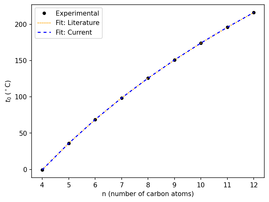
Now we plot both fits over the data. The fits are indistinguishable in this view.
seaborn.lineplot(data=df_linear_alkanes, x="n", y="t0_obs °C", label='Experimental', marker='o', linestyle='', color="black")
seaborn.lineplot(data=df_linear_alkanes, x='n', y='t0_calc', color='orange', dashes=[1], label='Fit: Literature')
seaborn.lineplot(data=df_linear_alkanes, x='n', y='t0_calc_current', color='blue', dashes=[3], label='Fit: Current')

plt.xlabel(n_label)
plt.ylabel(t0_label)
Text(0, 0.5, '$t_{0}$ ($^\\circ$C)')

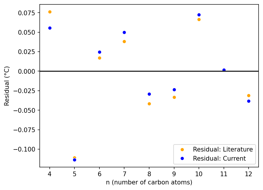
To check for any small differences in the fits, we calculate and plot the residuals.
df_linear_alkanes = df_linear_alkanes.with_columns(
    [
        pl.struct(["t0_calc", "t0_obs °C"])
        .apply(lambda x: x["t0_calc"] - x["t0_obs °C"])
        .alias("residuals_lit"),
        pl.struct(["t0_calc_current", "t0_obs °C"])
        .apply(lambda x: x["t0_calc_current"] - x["t0_obs °C"])
        .alias("residuals_current"),
    ]
)
seaborn.lineplot(data=df_linear_alkanes, x='n', y='residuals_lit', color='orange', marker='o', linestyle='', label='Residual: Literature')
seaborn.lineplot(data=df_linear_alkanes, x='n', y='residuals_current', color='blue', marker='o', linestyle='', label='Residual: Current')

plt.xlabel(n_label)
plt.ylabel("Residual (°C)")
plt.axhline(0, color='black')
<matplotlib.lines.Line2D at 0x7f55ec571310>

The residuals follow the same pattern for both fits and appear fairly comparable, with our fit having noticeably better residuals for some values of $n$ (4, 8, and 9) but worse for others ($n = 6, 7$).
Refitting Wiener’s Equation
To refit Wiener’s equation (eqn 4), we define the fitting function. In contrast with Egloff’s equation, which had only one independent variable ($n$), Wiener’s has three: n, $Δ\omega$, and Δp. To have scipy’s curve_fit fit a multidimensional equation, we pass it the independent variables as a tuple X. For clarity, we unpack that tuple in the funtion. The other two function arguments are the parameters to be fit, k and b, which are the factors for Δomega and Δp respectively.
# Define the fitting function
def wiener_parametrized(X: Iterable, k: float, b: float) -> float:
    """
    Parametrized version to model Δt as (k/n^2)*Δomega + b*Δp
    https://pubs.acs.org/doi/pdf/10.1021/j150402a006
    :returns: Δt, difference in boiling point between alkane and its structral isomer of a linear alkane
    :param X: iterable (e.g. tuple or list) of n, Δomega, Δp
    :param k: number to multiply Δomega/n^2 by; Wiener found to be 5.5
    :param b: number to multiply Δp by; Wiener found to be 98
    """
    n, Δomega, Δp = X
    Δt = (k / np.square(n)) * Δomega + (b * np.array(Δp))
    return Δt
For this dataframe, we use an Apache Parquet file. Parquet files are column-oriented so they are efficient for filtering on a given column, rather than having to read all row records as in a CSV file. In this case, we chose Parquet for variety.
df = pl.read_parquet("/content/drive/MyDrive/data/wiener.parquet")
As with the other equation, we extract columns from the dataframe, then fit the data using the fitting function.
Δt_obs_list = df.select("Δt_obs °C").get_columns()[0].to_list()
n_list = df.select("n").get_columns()[0].to_list()
Δomega_list = df.select("Δomega").get_columns()[0].to_list()
Δp_list = df.select("Δp").get_columns()[0].to_list()
parameters_current_wiener, covariance_wiener = curve_fit(
    wiener_parametrized, (n_list, Δomega_list, Δp_list), Δt_obs_list, (100, 6)
)
k_current, b_current = parameters_current_wiener
b_current = float(b_current)
k_current
94.77479126048236
b_current
5.294131964069949
r_squared_current = r_squared(wiener_parametrized, (n_list, Δomega_list, Δp_list), Δt_obs_list, (k_current, b_current))
r_squared_current
0.9559936865110978
parameters_wiener_lit_raw = [98.0, 5.5]
parameters_wiener_lit = [np.float32(entry) for entry in parameters_wiener_lit_raw]
k_lit, b_lit = [np.float32(entry) for entry in parameters_wiener_lit]
r_squared_lit = r_squared(wiener_parametrized, (n_list, Δomega_list, Δp_list), Δt_obs_list, (k_lit, b_lit))
r_squared_lit
0.9517163368871863
r_squared_improvement = r_squared_current - r_squared_lit
r_squared_improvement
0.004277349623911575
Here our fit is more noticeably better than the literature, though the improvement is still small.
To calculate the model values and their residuals for each fit, we add columns to the Polars dataframe.
df = df.with_columns(
    [
        pl.struct(["n", "Δomega", "Δp"])
        .apply(lambda x: wiener_parametrized((x["n"], x["Δomega"], x["Δp"]), k_lit, b_lit))
        .alias("Δt_calc_lit °C"),
        pl.struct(["n", "Δomega", "Δp"])
        .apply(lambda x: wiener_parametrized((x["n"], x["Δomega"], x["Δp"]), k_current, b_current))
        .alias("Δt_calc_current °C"),
    ]
)
df = df.with_columns(
    [
        pl.struct(["Δt_obs °C", "Δt_calc_lit °C"])
        .apply(lambda x: x["Δt_obs °C"] - x["Δt_calc_lit °C"])
        .alias("Δt_residual_lit °C"),
        pl.struct(["Δt_obs °C", "Δt_calc_current °C"])
        .apply(lambda x: x["Δt_obs °C"] - x["Δt_calc_current °C"])
        .alias("Δt_residual_current °C"),
    ]
)
Let’s sample the first five rows of the dataframe:
df.select(
    ["n", "molecule", "t_obs °C", "Δt_obs °C", "Δt_calc_lit °C", "Δt_calc_current °C", "Δt_residual_lit °C", "Δt_residual_current °C", "Δomega", "Δp"]
).limit(5)
| n | molecule | t_obs °C | Δt_obs °C | Δt_calc_lit °C | Δt_calc_current °C | Δt_residual_lit °C | Δt_residual_current °C | Δomega | Δp |
|---|---|---|---|---|---|---|---|---|---|
| i64 | str | f64 | f64 | f64 | f64 | f64 | f64 | i64 | i64 |
| 4 | "n-Butane" | -0.5 | 0.0 | 0.0 | 0.0 | 0.0 | 0.0 | 0 | 0 |
| 4 | "2-Methylpropan… | -11.7 | 11.2 | 11.625 | 11.217556 | -0.425 | -0.017556 | 1 | 1 |
| 5 | "n-Pentane" | 36.1 | 0.0 | 0.0 | 0.0 | 0.0 | 0.0 | 0 | 0 |
| 5 | "2-Methylbutane… | 27.9 | 8.2 | 7.84 | 7.581983 | 0.36 | 0.618017 | 2 | 0 |
| 5 | "2,2-Dimethylpr… | 9.5 | 26.6 | 26.68 | 25.752231 | -0.08 | 0.847769 | 4 | 2 |
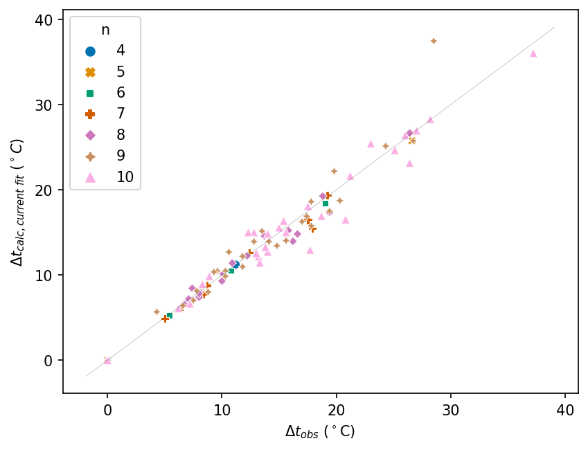
We can extract plot the current fit against the experimental Δt values. (You can find analogous plots for the literature fits in my original blog post Revisiting a Classic Cheminformatics Paper: The Wiener Index).
seaborn.scatterplot(
    data=df, x="Δt_obs °C", y="Δt_calc_current °C", hue="n", palette="colorblind", style="n"
)

plt.xlabel(Δt_obs_label)
plt.ylabel(Δt_calc_current_label)

# Add an equality line representing perfect predictions
#   Set its range using plot's range
x_range = plt.xlim()
y_range = plt.xlim()
equality_range = (min(x_range[0], y_range[0]), max(x_range[1], y_range[1]))

plt.plot(equality_range, equality_range, color="black", linewidth=0.1)
[<matplotlib.lines.Line2D at 0x7f55dfadfe50>]

The mol_frame package lets us show the molecules as pop-ups (tooltips) when we mouse over each data point. We will reproduce each plot as a mol_frame plot. For mol_frame, we have to convert the dataframe from Polars to pandas.
Unfortunately, the interactive plots are not working in the blog version of this notebook. Please visit the Google Colab notebook to access the interactive plot.
# Prepare dataframe for plotting with mol_frame
df_pandas = df.to_pandas()
df_mf = mf.MolFrame(df_pandas)
df_mf = df_mf.add_b64()
* using Smiles
* add b64:               (   94 |   31)
%%output filename="df_mol_frame_scatter"
hv.extension('bokeh')
df_mf.scatter("Δt_obs °C", "Δt_calc_current °C", colorby="n")
* using Mol_b64
* add img:               (   94 |   32)
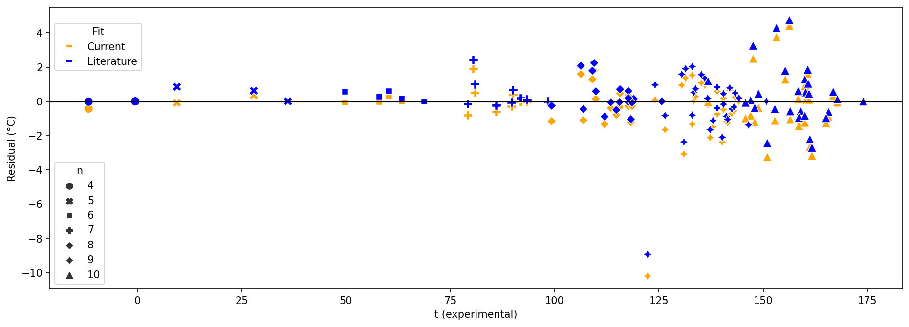
We next prepare to plot the residuals for both fits. It is challenging to plot multidimensional data: there is no obvious single x-axis coordinate to resolve all the molecules because no one of the independent variables $n$, $\Delta\omega$, and $\Delta p$ is unique for each molecule. We choose $t_{obs}$ because that value typically differs by molecule. We use a wide figure to help spatially resolve molecules with similar experimental $\Delta t$ values. We also vary the marker shape by $n$ to make it easier to visually match up pairs of data points (current vs. literature fit) corresponding to the same molecule.
# Make figure wide to help spatially resolve molecules with similar experimental Δt values
plt.figure(figsize=(15,5))

colors = ['orange', 'blue']
marker_size = 80

lit_fit = seaborn.scatterplot(
    data=df,
    x="t_obs °C",
    y="Δt_residual_lit °C",
    style="n",
    color=colors[0],
    s=marker_size,
)

current_fit = seaborn.scatterplot(
    data=df,
    x="t_obs °C",
    y="Δt_residual_current °C",
    style="n",
    # Suppress legend because it duplicates markers for other plot
    legend = False,
    color=colors[1],
    s=marker_size,
)

plt.axhline(0, color='black')
plt.xlabel("t (experimental)")
plt.ylabel("Residual (°C)")

# Prepare second legend with fit colors
fit_labels = ["Current", "Literature"]

# Create a list of Line2D objects with different colors
fit_handles = []
for i in range(len(fit_labels)):
    fit_handles.append(Line2D([0], [0], linestyle='none',
                              marker='_',
                              markeredgecolor=colors[i],
                              markeredgewidth=2,
                              ))

# Create a new legend for the fit variable
fit_legend = plt.figlegend(fit_handles, fit_labels, title="Fit",
                           loc="upper left",
                           bbox_to_anchor=(0.125, 0.85)
                           )

Here is the molframe version of the plot so you can tell which molecule corresponds to each data point.
%%output filename="df_mol_frame_residuals"
hv.extension('bokeh')
df_mf.scatter("t_obs °C", "Δt_residual_current °C", colorby="n")
* using Mol_b64
* add img:               (   94 |   32)
Reviewing each pair of points for the two fits on the seaborn scatter plot, again it is not obvious by inspection that the current fit is better than Wiener’s. The current fit generally seems to have a greater (more positive) value for each residual. We can sample the dataframe (excluding linear alkanes) to spot-check that, and notice that’s because the current fit yields slightly lesser (more negative) values for $Δt$.
df.filter((pl.col("Δomega") != 0) | (pl.col("Δp") != 0)).select(
    ["n", "molecule", "Δt_obs °C", "Δt_calc_lit °C", "Δt_calc_current °C", "Δt_residual_lit °C", "Δt_residual_current °C", "Δomega", "Δp"]
).limit(10)
| n | molecule | Δt_obs °C | Δt_calc_lit °C | Δt_calc_current °C | Δt_residual_lit °C | Δt_residual_current °C | Δomega | Δp |
|---|---|---|---|---|---|---|---|---|
| i64 | str | f64 | f64 | f64 | f64 | f64 | i64 | i64 |
| 4 | "2-Methylpropan… | 11.2 | 11.625 | 11.217556 | -0.425 | -0.017556 | 1 | 1 |
| 5 | "2-Methylbutane… | 8.2 | 7.84 | 7.581983 | 0.36 | 0.618017 | 2 | 0 |
| 5 | "2,2-Dimethylpr… | 26.6 | 26.68 | 25.752231 | -0.08 | 0.847769 | 4 | 2 |
| 6 | "2-Methylpentan… | 8.5 | 8.166667 | 7.897899 | 0.333333 | 0.602101 | 3 | 0 |
| 6 | "3-Methylpentan… | 5.4 | 5.388889 | 5.2364 | 0.011111 | 0.1636 | 4 | -1 |
| 6 | "2,2-Dimethylbu… | 19.0 | 19.055556 | 18.428432 | -0.055556 | 0.571568 | 7 | 0 |
| 6 | "2,3-Dimethylbu… | 10.8 | 10.833333 | 10.501667 | -0.033333 | 0.298333 | 6 | -1 |
| 7 | "2-Methylhexane… | 8.4 | 8.0 | 7.736718 | 0.4 | 0.663282 | 4 | 0 |
| 7 | "3-Methylhexane… | 6.5 | 6.5 | 6.310945 | 0.0 | 0.189055 | 6 | -1 |
| 7 | "3-Ethylpentane… | 5.0 | 5.0 | 4.885171 | 0.0 | 0.114829 | 8 | -2 |