Why some organic molecules have a color: Correlating optical absorption wavelength with conjugated bond chain length
Molecules have a color if their electronic energy levels are close enough to absorb visible rather than ultraviolet light. For organic molecules, that’s often because of an extensive chain of conjugated bonds. Can we use cheminformatics to find evidence that increasing conjugated bond chain length decreases absorption wavelength, which makes a molecule colored?
Open this notebook in Google Colab so you can run it without installing anything on your computer
Introduction
Colored molecules have applications in television screens, sensors, and to give color to fabrics, paints, foods, and more. I did my PhD in optical spectroscopy, so I was interested by the open-access database Experimental database of optical properties of organic compounds with more than 20,000 data points. One of the first things that came to mind was that organic colored compounds often get their color from an extensive chain of conjugated bonds. Here are quotes from an online textbook:
If you extend this to compounds with really massive delocalisation, the wavelength absorbed will eventually be high enough to be in the visible region of the spectrum, and the compound will then be seen as colored. A good example of this is the orange plant pigment, beta-carotene - present in carrots, for example.
The more delocalization there is, the smaller the gap between the highest energy pi bonding orbital and the lowest energy pi anti-bonding orbital. To promote an electron therefore takes less energy in beta-carotene than in the cases we’ve looked at so far - because the gap between the levels is less.
Here are two examples of molecules, one cyclic and one acylic, with conjugated pi bonds. In each case, the p orbitals on adjacent atoms line up so that the electrons are delocalized over all the conjugated bonds in the molecule (which is all the bonds in these two molecules).
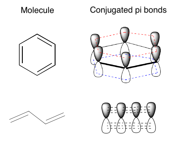
Attribution: Conjugated Pi Bond Systems from LibreTexts, remixed by Jeremy Monat
The more bonds that electrons can delocalize over, the more pi bonding and anti-bonding orbitals; and the highest occupied molecular orbital (HOMO, the top green line in each diagram below, the highest-energy pi bonding orbital) increases in energy, while the lowest unoccupied molecular orbital (LUMO, the lowest red line in each diagram below, the lowest-energy pi anti-bonding orbital) decreases in energy. The gap between the two becomes smaller, and if the conjugated chain is long enough, the HOMO-LUMO energy gap becomes small enough that it’s in the visible spectrum rather than the ultraviolet. When a molecule absorbs visible light, we perceive that it has a color.
Attribution: What Causes Molecules to Absorb UV and Visible Light from LibreTexts, authored, remixed, and/or curated by Jim Clark.
The visible spectrum starts at about 400 nm (violet) and goes to about 740 nm (red). So a molecule that absorbs light in that range will be perceived as colored.

Attribution: Gringer, Public domain, via Wikimedia Commons.
Cheminformatics exploration
Can we use cheminformatics to find evidence that increasing conjugated bond chain length decreases absorption wavelength? To check, I used the open-access database Experimental database of optical properties of organic compounds from 2020 with >20,000 chromophore-solvent combinations. The optical data can be downloaded as a CSV file (version 3).
Packages setup
import math
from typing import Iterable, Dict, List, Tuple
from IPython.display import display, Math
from functools import cache
import warnings

from PIL import Image
from rdkit import Chem
from rdkit.Chem import AllChem, Draw, Mol
import numpy as np
import polars as pl
import polars.selectors as cs
from polars.exceptions import ColumnNotFoundError
import altair as alt
from great_tables import GT, style, loc
import latexify
# Suppress the specific RDKit IPythonConsole truncation warning for MolsToGridImage
warnings.filterwarnings(
    "ignore", message=r"Truncating the list of molecules to be displayed to \d+"
)
Find longest conjugated bond chain
To find the longest conjugated bond chain in each molecule, we’ll use a graph-traversal algorithm. We’ll define two functions–one to find connected bonds and one to get the longest conjugated bond chain in a molecule–then describe how they work using an example molecule.
def find_connected_bonds(
    graph: np.ndarray,
    start_bond: int,
    visited: Iterable,
) -> List:
    """
    Find connected bonds in an adjacency matrix. Terminology is specific to bonds in molecules, but algorithm should work for any adjacency matrix.

    :param graph: The bond adjacency matrix
    :param start_bond: The bond index to start the chain from
    :param visited: The bond indices already visited; preferably a set for efficiency
    :returns: The list of bonds connected to, and including, the start bond
    """
    # Initialize the stack with the start bond
    stack = [start_bond]
    connected_component = []

    while stack:
        # Pop off the stack the last bond added
        bond_index = stack.pop()
        # Only follow the chain from this bond if this bond hasn't already been visited
        if bond_index not in visited:
            # Add the bond index to the list of visited bonds
            visited.add(bond_index)
            # Note that the bond is connected to the start bond
            connected_component.append(bond_index)

            # Add all neighbors to the stack for traversal if they haven't already been visited
            for neighbor, is_connected in enumerate(graph[bond_index]):
                if is_connected and neighbor not in visited:
                    stack.append(neighbor)
    return connected_component
def get_longest_conjugated_bond_chain(
    mol: Mol, verbose: bool = False
) -> tuple[List[int], np.ndarray]:
    """
    Get the longest conjugated bond chain in a molecule.

    :param mol: The RDKit molecule
    :param verbose: Whether to return the bond_matrix in addition to conjugated_bonds_out
    :returns: The list of bond indices of the longest conjugated bond chain in the molecule; if verbose is true, also the bond adjacency matrix
    """
    # Create a list to store conjugated bond indices
    conjugated_bonds = [
        bond.GetIdx() for bond in mol.GetBonds() if bond.GetIsConjugated()
    ]

    if not conjugated_bonds:
        # No conjugated bonds found, return empty list
        return []

    n_conjugated_bonds = len(conjugated_bonds)

    # Build a subgraph of the conjugated bonds only;
    #   initially populate it with zeroes, indicating bonds are not connected
    bond_matrix = np.zeros((n_conjugated_bonds, n_conjugated_bonds), dtype=int)

    # Populate the bond adjacency matrix for conjugated bonds
    for i, bond_i in enumerate(conjugated_bonds):
        bond_i_obj = mol.GetBondWithIdx(bond_i)
        # Avoid duplicate work by only processing pairs where j < i
        for j, bond_j in enumerate(conjugated_bonds[:i]):
            bond_j_obj = mol.GetBondWithIdx(bond_j)
            # Check if two conjugated bonds share an atom--
            #   do the set of {beginning atom, ending atom} overlap for the two bonds
            if {bond_i_obj.GetBeginAtomIdx(), bond_i_obj.GetEndAtomIdx()} & {
                bond_j_obj.GetBeginAtomIdx(),
                bond_j_obj.GetEndAtomIdx(),
            }:
                # Change the bond matrix value to 1, indicating the two bonds are connected
                bond_matrix[i, j] = 1
                bond_matrix[j, i] = 1

    # Initialize variables to store the longest conjugated bond chain
    visited = set()
    longest_bond_chain = []

    # Starting from each bond, traverse the graph and find the largest connected component
    for start_bond in range(n_conjugated_bonds):
        if start_bond not in visited:
            bond_chain = find_connected_bonds(bond_matrix, start_bond, visited)
            # Note that bonds are added to `visited` in find_connected_bonds(),
            #   so any bonds already visited from a previous starting bond
            #   won't have find_connected_bonds run on it
            # If this chain is longer than the longest one found so far, mark this chain as the longest
            if len(bond_chain) > len(longest_bond_chain):
                longest_bond_chain = bond_chain

    # Convert subgraph bond indices back to the original bond indices
    conjugated_bonds_out = [conjugated_bonds[i] for i in longest_bond_chain]
    conjugated_bonds_out.sort()

    if not verbose:
        return conjugated_bonds_out
    else:
        return conjugated_bonds_out, bond_matrix
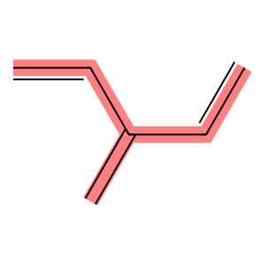
Let’s use an example branched molecule to explain how these algorithms work.
C6H8 = Chem.MolFromSmiles("C=CC(=C)C=C")
longest_conjugated_bond_chain, bond_matrix = get_longest_conjugated_bond_chain(
    mol=C6H8, verbose=True
)
Draw.MolToImage(
    C6H8,
    highlightBonds=longest_conjugated_bond_chain,
)
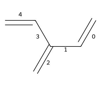
Let’s label the bond indices using RDKit’s addBondIndices.
opts = Draw.MolDrawOptions()
opts.addBondIndices = True
Draw.MolToImage(C6H8,size=(350,300),options=opts)
To understand the bond adjacency matrix, let’s use Polars’ Great Tables integration to make a nicely-formatted table.
# Convert the bond matrix to a Polars DataFrame
df_bond_matrix = pl.DataFrame(bond_matrix)

# Rename columns to add custom labels
df_bond_matrix = df_bond_matrix.rename(
    {f"column_{str(i)}": f"Bond {i}" for i in range(bond_matrix.shape[1])}
)

# Add row index labels (Polars doesn't have an index column, so we'll add it as a new column)
row_indices = [f"Bond {i}" for i in range(bond_matrix.shape[0])]
index_col = "Adjacent?"
df_bond_matrix = df_bond_matrix.insert_column(0, pl.Series(index_col, row_indices))

# Add a Total column to sum up how many bonds a given bond is connected to
total_col = "Total"
df_bond_matrix = df_bond_matrix.with_columns(
    pl.sum_horizontal(cs.starts_with("Bond")).alias(total_col)
)

# Use GreatTables to format the table
GT(df_bond_matrix).tab_options(
    # Bold the column headings
    column_labels_font_weight="bold",
).tab_style(
    # Bold the index and total columns
    style=style.text(weight="bold"),
    locations=loc.body(columns=[index_col, total_col]),
).tab_header(
    # Add a title to the table
    title="Bond adjacency matrix"
)
| Bond adjacency matrix | ||||||
| Adjacent? | Bond 0 | Bond 1 | Bond 2 | Bond 3 | Bond 4 | Total |
|---|---|---|---|---|---|---|
| Bond 0 | 0 | 1 | 0 | 0 | 0 | 1 |
| Bond 1 | 1 | 0 | 1 | 1 | 0 | 3 |
| Bond 2 | 0 | 1 | 0 | 1 | 0 | 2 |
| Bond 3 | 0 | 1 | 1 | 0 | 1 | 3 |
| Bond 4 | 0 | 0 | 0 | 1 | 0 | 1 |
The table demonstrates which bonds are adjacent, in the sense that the two bonds share an atom. For example, bond 1 is adjacent to bonds 0, 2, and 3. That makes sense based on the molecular diagram.
The bond chain starts with a start bond, in this case 0, and follows all its adjacent bonds to make a chain. Here, the algorithm went to bond 1 (the only bond connected to bond 0), then at the branch chose to go off the molecule’s spine (longest atom chain) to go to bond 2, then followed the other branch to complete the molecule’s spine (bonds 3 and 4):
longest_conjugated_bond_chain
[0, 1, 2, 3, 4]
In this case, a single bond chain found all the conjugated bonds in the molecule. The algorithm loops over all conjugated bonds to make sure it finds the longest chain. But if a given start bond (e.g., 1) was already visited because it was in the bond chain of a previous starting bond (e.g., 0), the algorithm doesn’t re-trace the same bond chain. This is a big computational savings because it avoids unnecessary graph traversals, which are expensive. This is facilitated by the variable visited being passed from get_longest_conjugated_bond_chain() to find_connected_bonds(), where it is modified by adding the nodes visited.
Additional computational savings comes from excluding the non-conjugated bonds from the adjacency matrix. While not noticeable for the example molecule because all its bonds are conjugated, this can greatly reduce the adjacency matrix, and thus the graph traversal, for molecules where some bonds are not conjugated.
Check that longest conjugated bond chain gives expected results
Let’s make sure that our algorithm gives the expected results for a variety of cyclic and acyclic molecules.
examples = {
    "benzene": "c1ccccc1",
    "naphthalene": "c1c2ccccc2ccc1",
    "anthracene": "c1ccc2cc3ccccc3cc2c1",
    "toluene": "c1ccccc1C",
    "benzene + 5 linear conjugated bonds": "c1ccccc1CC=CC=CC=C",
    "benzene + 7 linear conjugated bonds": "c1ccccc1CC=CC=CC=CC=C",
    "1,3-butadiene": "C=CC=C",
    "branched": "C=C\C=C/C(/C=C)=C/C=C",
    "branched + distant": "C=C\C=C\C\C=C\C=C/C(/C=C)=C/C=C",
}
mols = [Chem.MolFromSmiles(sml) for sml in examples.values()]
conjugated_bonds = [get_longest_conjugated_bond_chain(mol) for mol in mols]
Draw.MolsToGridImage(
    mols=mols,
    legends=examples.keys(),
    highlightBondLists=conjugated_bonds,
    subImgSize=(300, 200),
)
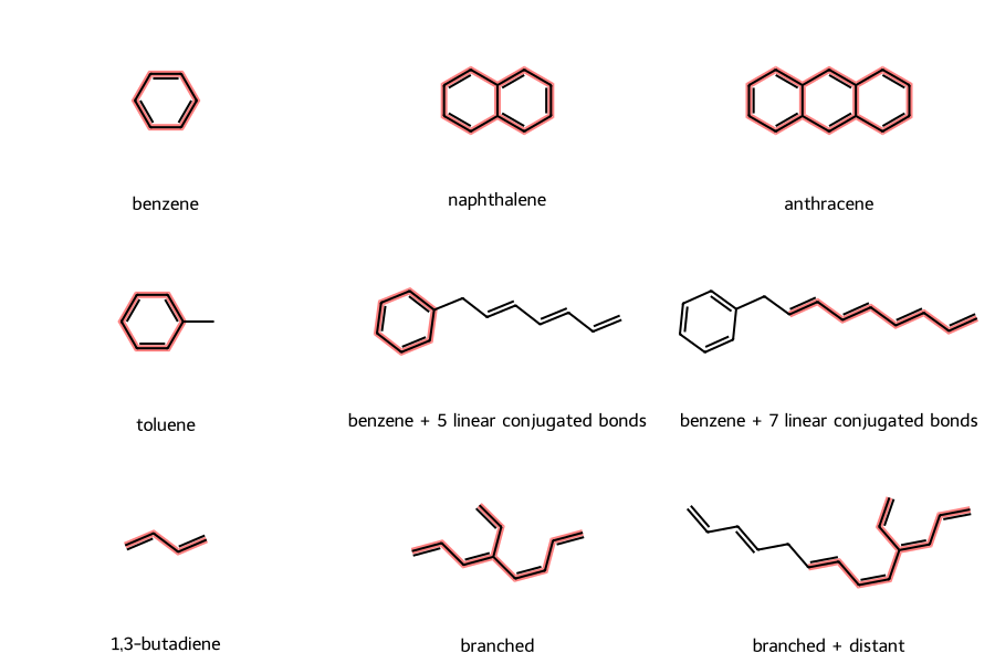
Those highlighted conjugated bond chains are as expected, for example
- all the bonds are conjugated in benzene, as well as fused polycyclic molecules naphthalene and anthracene
- the bond off the ring in toluene is not conjugated
- if we put a side-chain on benzene with fewer than six conjugated bonds, the benzyl moiety remains the longest conjugated chain; but if we have seven conjugated bonds on the side chain, it becomes the longest conjugated chain
- in the “branched + distant” molecule, if we break the conjugation chain by having two C-C single bonds in a row, the chain does not include the distant, disconnected conjugated bonds
Of course we should check beta-carotene, whose color comes from its extended conjugated bond chain and is “responsible for the orange color of carrots”. beta-carotene “absorbs most strongly between 400-500 nm. This is the green/blue part of the spectrum.” Because it absorbs those wavelengths, when we look at a sample of beta-carotene we see the reflected light of the complimentary colors, so we perceive an orange color. Note that beta-carotene’s absorption isn’t that much lower energy (higher wavelength) than ultraviolet (which goes up to 400 nm), so molecules with longer conjugated chains might absorb at higher wavelengths such as 565-590 nm (yellow), giving them perceived colors towards blue, magenta, and purple.
beta_carotene = Chem.MolFromSmiles(
    "CC2(C)CCCC(\C)=C2\C=C\C(\C)=C\C=C\C(\C)=C\C=C\C=C(/C)\C=C\C=C(/C)\C=C\C1=C(/C)CCCC1(C)C"
)
longest_conjugated_bond_chain = get_longest_conjugated_bond_chain(beta_carotene)
print(
    f"beta-carotene's longest conjugated bond chain is {len(longest_conjugated_bond_chain)} bonds long."
)
Draw.MolToImage(
    beta_carotene,
    highlightBonds=longest_conjugated_bond_chain,
    size=(800, 200),
)
beta-carotene's longest conjugated bond chain is 21 bonds long.
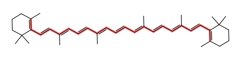
And beta-carotene’s molecular structure is also beautifully symmetric.
Now that we have an algorithm to find the longest conjugated bond chain in a molecule, let’s apply it to the optical dataset.
Prepare data
Let’s read into a Polars dataframe the data from the optical dataset CSV file.
df = pl.read_csv("../data/DB for chromophore_Sci_Data_rev03.csv")

# If there are any rows where all values are null, drop those rows
df = df.filter(~pl.all_horizontal(pl.all().is_null()))

df
| Tag | Chromophore | Solvent | Absorption max (nm) | Emission max (nm) | Lifetime (ns) | Quantum yield | log(e/mol-1 dm3 cm-1) | abs FWHM (cm-1) | emi FWHM (cm-1) | abs FWHM (nm) | emi FWHM (nm) | Molecular weight (g mol-1) | Reference |
|---|---|---|---|---|---|---|---|---|---|---|---|---|---|
| i64 | str | str | f64 | f64 | f64 | f64 | f64 | f64 | f64 | f64 | f64 | f64 | str |
| 0 | "N#Cc1cc2ccc(O)cc2oc1=O" | "O" | 355.0 | 410.0 | 2.804262 | null | null | null | null | null | null | 187.026943 | "10.1021/acs.jpcb.5b09905" |
| 1 | "N#Cc1cc2ccc([O-])cc2oc1=O" | "O" | 408.0 | 450.0 | 3.961965 | null | null | null | 2128.3 | null | 43.2 | 186.019667 | "10.1021/acs.jpcb.5b09905" |
| 2 | "CCCCCCCCCCCC#CC#CCCCCCCCCCN1C(… | "ClC(Cl)Cl" | 526.0 | 535.0 | 3.602954 | null | null | null | null | null | null | 1060.705709 | "10.1002/smll.201901342" |
| 3 | "[O-]c1c(-c2nc3ccccc3s2)cc2ccc3… | "CC#N" | 514.0 | 553.7 | 3.81 | null | null | null | 2120.5 | null | 65.2 | 350.064509 | "10.1016/j.snb.2018.10.043" |
| 4 | "[O-]c1c(-c2nc3ccccc3s2)cc2ccc3… | "CS(C)=O" | 524.0 | 555.0 | 4.7 | null | null | 2219.7 | 1565.6 | 61.2 | 48.3 | 350.064509 | "10.1016/j.snb.2018.10.043" |
| … | … | … | … | … | … | … | … | … | … | … | … | … | … |
| 20831 | "N#Cc1c(N2CCCCC2)cc(-c2ccc3ccc4… | "C1CCOC1" | 344.0 | 473.0 | null | null | null | null | 3937.1 | null | 88.9 | 488.188863 | "10.1021/ol9000679" |
| 20832 | "CCCCCCn1c2c(c3ccccc31)-c1c(c3c… | "ClCCl" | 312.0 | 352.0 | null | null | 4.460898 | null | null | null | null | 797.18392 | "DOI: 10.1021/ol501083d" |
| 20833 | "CCCCCCn1c2c(c3cc(-c4ccc5ccc6cc… | "ClCCl" | 340.0 | 382.0 | null | null | 4.70757 | null | null | null | null | 1598.142 | "DOI: 10.1021/ol501083d" |
| 20834 | "CCCCCCn1c2c(c3ccccc31)-c1c(c3c… | "CCCCCCn1c2c(c3ccccc31)-c1c(c3c… | 321.0 | 494.0 | null | null | null | null | null | null | null | 797.18392 | "DOI: 10.1021/ol501083d" |
| 20835 | "CCCCCCn1c2c(c3cc(-c4ccc5ccc6cc… | "CCCCCCn1c2c(c3cc(-c4ccc5ccc6cc… | 365.0 | 466.0 | null | null | null | null | null | null | null | 1598.142 | "DOI: 10.1021/ol501083d" |
The dataset gives absorption and emission maxima as wavelengths. That makes sense because spectroscopists wavelength describes the color of the light used in the laboratory. But to compare, for example, the absorption and emission maximum for a molecule, it’s better to use energy units to express the difference between different molecular energy levels. So let’s convert wavelengths to energies in electron volts, eV.
To determine the conversion factor, let’s use the equation for energy E as a function of wavelength λ.
@latexify.function
def E(
    h: float,
    c: float,
    λ: float,
) -> float:
    """Calculate the binomial coefficient: how many ways there are to choose k items from n items.

    :param h: Planck's constant
    :param c: speed of light
    :param λ: wavelength
    :returns: energy
    """
    return h * c / λ


E
Let’s plug in the values of the physical constants to four decimal places and use factor-label dimensional analysis:
eqn = r"$E = \frac{6.6261 \times 10^{-34} \, \text{J} \cdot \text{s} \cdot 2.9979 \times 10^8 \, \text{m/s}}{\lambda \times 10^{-9} \, \text{m}} \cdot \frac{1 \, \text{eV}}{1.6022 \times 10^{-19} \, \text{J}} = \frac{1239.8 \, \text{eV}}{\lambda}$"
display(Math(eqn))
$\displaystyle E = \frac{6.6261 \times 10^{-34} \, \text{J} \cdot \text{s} \cdot 2.9979 \times 10^8 \, \text{m/s}}{\lambda \times 10^{-9} \, \text{m}} \cdot \frac{1 \, \text{eV}}{1.6022 \times 10^{-19} \, \text{J}} = \frac{1239.8 \, \text{eV}}{\lambda}$
Doing that in Python to store the value in a variable:
h = 6.6261e-34  # J*s
c = 2.9979e8  # m/s
nm = 1e-9  # m
eV = 1.6022e-19  # J
eV_nm = h * c / (nm * eV)
eV_nm
1239.8193228061414
Now we can convert absorption and emission maxima to energy units of eV, then calculate their difference as the Stokes shift. The Stokes shift reflects how much the molecule relaxes from its initial excited state (the Franck–Condon state) to the lowest vibrational level in the excited state that it typically emits light from. In the following diagram, the blue arrow represents absorption from the ground state to the Franck-Condon state, and the green arrow represents emission from the relaxed excited state back to the ground state. The blue arrow is longer, representing the greater energy of absorption. The difference between the vertical length of the blue and green arrows is the Stokes shift.

Attribution: Franck Condon Diagram on Wikipedia by Samoza, licensed under the Creative Commons Attribution-Share Alike 3.0 Unported license
# To prevent duplicate-column errors when re-running this code, drop the columns we're about to add
for column in [
    "longest_bond_indices",
    "Longest conjugated bond length",
    "Absorption max (eV)",
    "Emission max (eV)",
    "Stokes shift (eV)",
]:
    try:
        df.drop(column)
    except ColumnNotFoundError:
        pass
Now we can calculate the energies in eV from the wavelengths in nm.
df = df.with_columns(
    [
        (eV_nm / pl.col("Absorption max (nm)")).alias("Absorption max (eV)"),
        (eV_nm / pl.col("Emission max (nm)")).alias("Emission max (eV)"),
    ]
).with_columns(
    (pl.col("Absorption max (eV)") - pl.col("Emission max (eV)")).alias(
        "Stokes shift (eV)"
    ),
)
Finding the longest conjugated chain for each molecule
Now we come to the computationally-intensive operation: Finding the the longest conjugated chain for each molecule using conjugated_chain() which calls get_longest_conjugated_bond_chain(). We define a function that will return the indices and length of the longest conjugated bond chain. The data set repeats some chromophores: there are a little less than three rows per chromophore. So we’ll cache the results for each chromophore to avoid recalculating for each of its rows. Python’s built-in module functools include a cache decorator that makes this simple.
@cache
def conjugated_chain(sml) -> Dict[str : List[int], str:int]:
    """
    Find the indices and length for the longest bond chain in a SMILES.

    :param sml: SMILES to be made into a molecule
    :returns: A dictionary of longest bond chain indices and longest bond chain length
    """
    return_dict = dict()
    mol = Chem.MolFromSmiles(sml)
    longest_bond_indices = get_longest_conjugated_bond_chain(mol)
    return_dict["longest_bond_indices"] = longest_bond_indices
    return_dict["Longest conjugated bond length"] = len(longest_bond_indices)
    return return_dict
Now we use Polars’ map_elements to calculate the longest bond chain for each molecule. Because conjugated_chain() returns a dictionary, Polars treats it as a struct, which we can then unnest to create a column for each dictionary key-value pair. We then sort the dataframe to put the longest bond chain lengths first so we can examine those molecules. Finally, we use Polars’ shrink_to_fit() to decrease the dataframe memory usage and prevent problems with plotting.
This entire operation takes about 13 seconds on my laptop with caching, and about 33 seconds without, which roughly reflects the ratio of unique chromophores to data points. Caching is thus demonstrated to be effective here.
# This may take 12-60 seconds: Finding the longest conjugated chain in each molecule in the dataframe
df = (
    df.with_columns(
        conjugated=pl.col("Chromophore").map_elements(
            lambda sml: conjugated_chain(sml), return_dtype=pl.Struct
        )
    )
    .unnest("conjugated")
    .sort(pl.col("Longest conjugated bond length"), descending=True)
    .shrink_to_fit()
)
df.head()
| Tag | Chromophore | Solvent | Absorption max (nm) | Emission max (nm) | Lifetime (ns) | Quantum yield | log(e/mol-1 dm3 cm-1) | abs FWHM (cm-1) | emi FWHM (cm-1) | abs FWHM (nm) | emi FWHM (nm) | Molecular weight (g mol-1) | Reference | Absorption max (eV) | Emission max (eV) | Stokes shift (eV) | longest_bond_indices | Longest conjugated bond length |
|---|---|---|---|---|---|---|---|---|---|---|---|---|---|---|---|---|---|---|
| i64 | str | str | f64 | f64 | f64 | f64 | f64 | f64 | f64 | f64 | f64 | f64 | str | f64 | f64 | f64 | list[i64] | i64 |
| 16578 | "N#CC(C#N)=C1C=C(C=Cc2ccc(-c3cc… | "N#CC(C#N)=C1C=C(C=Cc2ccc(-c3cc… | null | 706.0 | null | 0.12 | null | null | null | null | null | 2731.043503 | "10.1039/c6tc03359h" | null | 1.756118 | null | [0, 1, … 242] | 243 |
| 16648 | "C(=Cc1ccc(C=Cc2ccc(N(c3ccc(-c4… | "C(=Cc1ccc(C=Cc2ccc(N(c3ccc(-c4… | null | 660.0 | null | null | null | null | null | null | null | 1994.81382 | "10.1039/c6tc03359h" | null | 1.878514 | null | [0, 1, … 177] | 178 |
| 16555 | "CC(C)c1cccc(C(C)C)c1N1C(=O)c2c… | "CC(C)c1cccc(C(C)C)c1N1C(=O)c2c… | null | 790.0 | null | null | null | null | null | null | null | 2094.857519 | "10.1039/c6tc03359h" | null | 1.569392 | null | [3, 4, … 185] | 174 |
| 16554 | "CC(C)c1cccc(C(C)C)c1N1C(=O)c2c… | "CC(C)c1cccc(C(C)C)c1N1C(=O)c2c… | null | 860.0 | null | null | null | null | null | null | null | 2030.87786 | "10.1039/c6tc03359h" | null | 1.44165 | null | [3, 4, … 181] | 170 |
| 15298 | "c1ccc(C(=C(c2ccccc2)c2ccc(-c3c… | "Cc1ccccc1" | 530.0 | 637.0 | null | 0.252 | null | null | null | null | null | 1760.698122 | "10.1016/j.dyepig.2012.08.028" | 2.339282 | 1.946341 | 0.392941 | [0, 1, … 157] | 158 |
Checking the results, we find that the longest conjugated bond chain length in the optical dataset is 158 bonds! That’s more than seven times longer than beta-carotene’s. So it certainly makes sense that some of these molecules absorb visible light. For example, the molecule with the longest conjugated bond chain has its absorption maximum at 530 nm in the solvent of toluene.
Checking for a correlation of absorption wavelength against longest conjugated bond chain length
Let’s use Polars’ plot capability to plot absorption max against longest bond length to check for any trends. Altair can plot a maximum of 5,000 data points, and there are more than 20,000 points in the optical dataset. We could enable VegaFusion to allow for more points, but that would be an additional dependency and it seems not to work well with Google Colab. Instead, let’s filter down to the ~7k unique chromophores in the dataset and plot the first 5k. Polars will select one solvent essentially at random for each chromophore, and the solvatochromic shift is generally not huge compared to the range we’ll be plotting (from <200 to 850 nm), so that’s a reasonable sampling. And 5k points should be plenty to discern if there’s a trend.
df_unique_chromophore = df.unique(subset="Chromophore")
We also need to drop the column longest_bond_indices because large lists of integers are not supported (we’re not plotting them anyway)
Now we can make a plot of absorption maximum against longest conjugated bond length for the first 5k unique chromophores.
df_unique_chromophore.slice(0, 5000).drop("longest_bond_indices").plot.scatter(
    x="Longest conjugated bond length", y="Absorption max (nm)"
)
There’s not much of a correlation, presumably because of the varied molecular structures.
Seeking a series of related molecules
Let’s remove other variables by finding a series of molecules with a similar structure, but where the longest conjugated bond chain length increases. Given our dataset, let’s start with molecules with a large number of connected conjugated bonds, then hopefully find a simple, linear molecule with a repeat unit that we can look for molecular analogues with fewer repeat units. We’ll plot the top 50 molecules, which is the RDKit’s default maximum for MolsToGridImage.
# Filter down to unique chromophores to avoid repeats in the molecular grid
df_unique_chromophore = df_unique_chromophore.sort(
    "Longest conjugated bond length", descending=True
)

# Extract columns as lists so we can plot molecules in a grid
unique_chromophores = df_unique_chromophore["Chromophore"].to_list()
tags = df_unique_chromophore["Tag"].to_list()
longest_conjugated_bond_lengths = df_unique_chromophore["Longest conjugated bond length"].to_list()
legends = [
    f"{longest_bond_length} bonds: tag {tag}"
    for (tag, longest_bond_length) in zip(tags, longest_conjugated_bond_lengths)
]
mols = [Chem.MolFromSmiles(chromophore) for chromophore in unique_chromophores]
Draw.MolsToGridImage(
    mols=mols,
    legends=legends,
    molsPerRow=5,
)
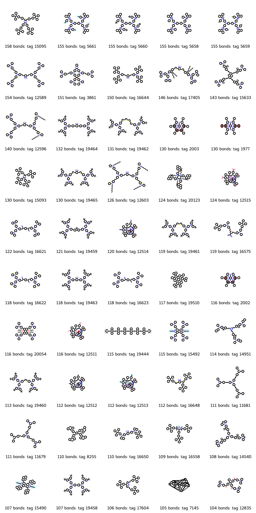
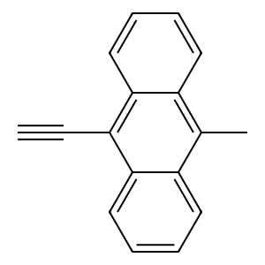
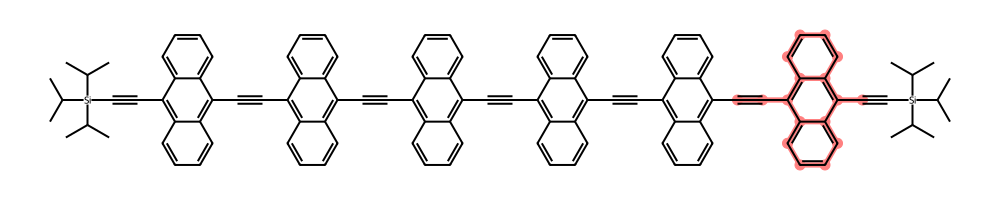
While there are a lot of interesting-looking molecules, tag 19940 has a simple linear structure with a clear repeat unit that includes an anthracene moiety. This molecule has six of those repeat units, so we’ll refer to it as the n = 6 molecule. Let’s show the molecule with its conjugated chain highlighted.
size_wide_mol = (1000, 200)
df_n6 = df_unique_chromophore.filter(Tag=19940)
sml_n6 = df_n6[0]["Chromophore"].item()
mol_n6 = Chem.MolFromSmiles(sml_n6)
tags = df_n6[0]["Tag"].item()
longest_bond_length = df_n6[0]["Longest conjugated bond length"].item()
legend = f"{longest_bond_length} bonds: tag {tags}"
conjugated_bonds_n6 = df_n6[0]["longest_bond_indices"].item().to_list()
Draw.MolToImage(
    mol=mol_n6,
    size=size_wide_mol,
    legend=legend,
    highlightBonds=conjugated_bonds_n6,
)
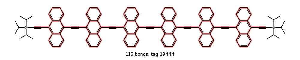
By the way, sometimes it’s difficult to see that all the specified bonds have been highlighted in the molecular image; there is in fact a contiguous chain from the first triple bond to the last.
Now let’s show the repeat unit in the same orientation as the molecule, which requires rotating the atoms of the repeat unit by 90 degrees. We’ll rotate serval molecules in this post by 90 degrees, so let’s define a function to do that.
def rotate_90(sml: str) -> Mol:
    """
    Rotates a molecule by 90 degrees based on its SMILES string and visualizes it.

    :param sml: SMILES string of the molecule to rotate.
    :returns: The rotated molecule.
    """

    mol = Chem.MolFromSmiles(sml)

    # Generate 2D coordinates if not already present
    AllChem.Compute2DCoords(mol)

    # Define the rotation matrix for 90 degrees (π/2 radians)
    theta = np.pi / 2  # 90 degrees in radians
    rotation_matrix = np.array(
        [[np.cos(theta), -np.sin(theta)], [np.sin(theta), np.cos(theta)]]
    )

    # Get the conformation of the molecule (the 2D coordinates)
    conf = mol.GetConformer()

    # Apply the rotation to each atom
    for i in range(mol.GetNumAtoms()):
        # Get the current x, y, z coordinates (z will stay 0.0 for 2D)
        pos = conf.GetAtomPosition(i)
        x, y = pos.x, pos.y  # Extract x, y coordinates

        # Apply the 90-degree rotation
        new_x, new_y = np.dot(rotation_matrix, [x, y])

        # Set the new coordinates, keeping z=0.0
        conf.SetAtomPosition(i, (new_x, new_y, 0.0))

    # Return the rotated molecule
    return mol
Now we can show the repeat unit in the same orientation that it appears in the n = 6 molecule. The RDKit tends to recalculate molecular coordinates, so to be safe we assign the output image of Draw.MolToImage to a variable, then display that image.
repeat_unit = "CC1=C2C=CC=CC2=C(C#C)C2=CC=CC=C12"
repeat_unit_mol = Chem.MolFromSmiles(repeat_unit)

repeat_unit_mol = rotate_90(repeat_unit)
image = Draw.MolToImage(
    repeat_unit_mol,
)
display(image)
Let’s check the dataframe for molecules with the same overall structure, with fewer repeat units. To do that, we’ll need to check for a substructure in a molecule.
Filter to molecules in the series
Let’s define a function to check how many of a given substructure there are in a molecule.
def match_counts(
    sml: str,
    smls_to_match: Iterable[str] = None,
) -> Dict[str, int]:
    """
    Convert target and to-match SMILES to RDKit molecules, then count how many times the to-match molecules occur in the target molecules.

    :param sml: SMILES to convert to a molecule
    :param smls_to_match: One or more SMILES to find as a substructure
    :returns: Dictionary with name:count entry for each SMILES to match
    """
    mol = Chem.MolFromSmiles(sml)
    return_dict = dict()
    for name, sml_to_match in smls_to_match.items():
        mol_to_match = Chem.MolFromSmiles(sml_to_match)
        matches = mol.GetSubstructMatches(mol_to_match)
        return_dict[f"{name}_match_count"] = len(matches)
    return return_dict
To prevent double-counting of the number of repeat units, we use a substructure one atom longer than we showed above.
smls_to_match = {
    # Repeat unit containing an anthracene moiety, with two triple bonds
    "repeat_unit": "C#CC1=C2C=CC=CC2=C(C#C)C2=CC=CC=C12",
}
Let’s highlight one instance of the repeat unit, and of the terminal group, in the n = 6 molecule. Because we’ll search by atoms (the substructure), and then want to highlight the bonds as well, we’ll define a function to get the bond indices connecting an iterable of atoms.
def get_bond_indices_connecting_atoms(
    mol: Mol, atom_indices: Iterable[int]
) -> List[int]:
    """
    Given an RDKit molecule and a list of atom indices, return the bond indices
    that connect the atoms in the list.

    :param mol: RDKit molecule object
    :param atom_indices: List of atom indices to check for connectivity
    :return: List of bond indices that connect the atoms in atom_indices
    """
    bond_indices = []
    atom_set = set(atom_indices)  # Using a set for faster lookup

    # Iterate through all bonds in the molecule
    for bond in mol.GetBonds():
        begin_atom = bond.GetBeginAtomIdx()
        end_atom = bond.GetEndAtomIdx()

        # Check if both atoms of the bond are in the provided list of atom indices
        if begin_atom in atom_set and end_atom in atom_set:
            bond_indices.append(bond.GetIdx())

    return bond_indices
# Get the first repeat unit substructure match
match_repeat_unit = mol_n6.GetSubstructMatches(repeat_unit_mol)[0]
bond_indices_repeat_unit = get_bond_indices_connecting_atoms(mol_n6, match_repeat_unit)
Draw.MolToImage(
    mol_n6,
    highlightAtoms=match_repeat_unit,
    highlightBonds=bond_indices_repeat_unit,
    size=size_wide_mol,
)
To avoid duplicate-column errors when the code is run more than once, we’ll drop any existing match count columns. Then we’ll count the occurrences of each substructure in each molecule.
def add_match_counts(
    df: pl.DataFrame,
    smls_to_match: Iterable[str],
) -> pl.DataFrame:
    """
    For a dataframe with SMILES, add the count of matching substructures for SMILES to match.

    :param df: Polars dataframe of molecules with SMILES in Chromophore column
    :param smls_to_match: Iterable of SMILES for substructures
    :returns: Polars dataframe with match count columns added
    """
    df = df.drop(cs.ends_with("_match_count"))
    df = (
        df.with_columns(
            substructure_counts=pl.col("Chromophore").map_elements(
                lambda sml: match_counts(sml, smls_to_match), return_dtype=pl.Struct
            )
        )
        .unnest("substructure_counts")
        .sort("Longest conjugated bond length", descending=True)
        .shrink_to_fit()
    )
    return df
df = add_match_counts(
    df=df,
    smls_to_match=smls_to_match,
)
Let’s filter down to molecules that contain the repeat unit by requiring the repeat unit match count be greater than zero.
df.filter((pl.col("repeat_unit_match_count") > 0)).sort(
    pl.col("repeat_unit_match_count")
)
| Tag | Chromophore | Solvent | Absorption max (nm) | Emission max (nm) | Lifetime (ns) | Quantum yield | log(e/mol-1 dm3 cm-1) | abs FWHM (cm-1) | emi FWHM (cm-1) | abs FWHM (nm) | emi FWHM (nm) | Molecular weight (g mol-1) | Reference | Absorption max (eV) | Emission max (eV) | Stokes shift (eV) | longest_bond_indices | Longest conjugated bond length | repeat_unit_match_count |
|---|---|---|---|---|---|---|---|---|---|---|---|---|---|---|---|---|---|---|---|
| i64 | str | str | f64 | f64 | f64 | f64 | f64 | f64 | f64 | f64 | f64 | f64 | str | f64 | f64 | f64 | list[i64] | i64 | i64 |
| 19379 | "CCCCCCCCn1c(=O)c2cc3c(C#Cc4ccc… | "ClC(Cl)Cl" | 582.0 | 641.0 | 3.4 | 0.53 | 4.518514 | null | 1387.6 | null | 57.1 | 1074.508407 | "10.1021/acs.joc.6b00364" | 2.130274 | 1.934196 | 0.196078 | [8, 9, … 91] | 76 | 1 |
| 19384 | "CCCCCCCCn1c(=O)c2cc3c(C#Cc4ccc… | "c1ccccc1" | 584.0 | 627.0 | null | null | null | null | null | null | null | 1074.508407 | "10.1021/acs.joc.6b00364" | 2.122978 | 1.977383 | 0.145595 | [8, 9, … 91] | 76 | 1 |
| 19388 | "CCCCCCCCn1c(=O)c2cc3c(C#Cc4ccc… | "C1CCOC1" | 563.0 | 641.0 | null | null | null | null | null | null | null | 1074.508407 | "10.1021/acs.joc.6b00364" | 2.202166 | 1.934196 | 0.26797 | [8, 9, … 91] | 76 | 1 |
| 20066 | "O=c1c2ccccc2c2nc3cc4c(C#C[Si](… | "ClCCl" | 731.0 | null | null | null | null | null | null | null | null | 1238.628931 | "10.1021/acs.joc.9b02756" | 1.696059 | null | null | [0, 1, … 107] | 64 | 1 |
| 20073 | "O=c1c2ccccc2c2nc3cc4c(C#C[Si](… | "O=c1c2ccccc2c2nc3cc4c(C#C[Si](… | 743.0 | null | null | null | null | null | null | null | null | 1238.628931 | "10.1021/acs.joc.9b02756" | 1.668667 | null | null | [0, 1, … 107] | 64 | 1 |
| … | … | … | … | … | … | … | … | … | … | … | … | … | … | … | … | … | … | … | … |
| 19936 | "CC(C)[Si](C#Cc1c2ccc(C(C)(C)C)… | "Cc1ccccc1" | 523.0 | 541.0 | null | 0.02 | 4.694605 | 3158.9 | 1770.3 | 87.0 | 51.9 | 962.658106 | "10.1021/acs.joc.8b00311" | 2.370591 | 2.291718 | 0.078874 | [4, 5, … 74] | 39 | 2 |
| 19937 | "CC(C)[Si](C#Cc1c2ccc(C(C)(C)C)… | "Cc1ccccc1" | 570.0 | 589.0 | null | 0.022 | 4.781037 | 3541.0 | 911.6 | 116.2 | 31.6 | 1274.845907 | "10.1021/acs.joc.8b00311" | 2.175122 | 2.104956 | 0.070165 | [4, 5, … 101] | 58 | 3 |
| 19938 | "CC(C)[Si](C#Cc1c2ccc(C(C)(C)C)… | "Cc1ccccc1" | 582.0 | 609.0 | null | 0.02 | 4.975432 | 3895.7 | 1206.4 | 133.7 | 44.8 | 1587.033707 | "10.1021/acs.joc.8b00311" | 2.130274 | 2.035828 | 0.094446 | [4, 5, … 128] | 77 | 4 |
| 19939 | "CC(C)[Si](C#Cc1c2ccc(C(C)(C)C)… | "Cc1ccccc1" | 585.0 | 623.0 | null | 0.018 | 5.130334 | 3751.8 | 1204.5 | 130.0 | 46.8 | 1899.221508 | "10.1021/acs.joc.8b00311" | 2.119349 | 1.990079 | 0.12927 | [4, 5, … 155] | 96 | 5 |
| 19940 | "CC(C)[Si](C#Cc1c2ccc(C(C)(C)C)… | "Cc1ccccc1" | 589.0 | 629.0 | null | null | 5.178977 | 3681.3 | 1318.7 | 129.2 | 52.3 | 2211.409309 | "10.1021/acs.joc.8b00311" | 2.104956 | 1.971096 | 0.133861 | [4, 5, … 182] | 115 | 6 |
That’s too many molecules–we expect as many as six, for n = 1-6. Let’s examine the molecular structures to understand why.
Because we’ll plot several instances of molecular grids from subsets of the dataframe, we define a function to plot first ten molecules and legends based on the columns in the dataframe.
def df_to_grid_image(
    df: pl.DataFrame,
    subImgSize: Tuple[int, int] = (200, 200),
    molsPerRow=3,
) -> Image.Image:
    """
    Create a molecular grid image from a Polars dataframe.

    :param df: Polars dataframe
    :param subImgSize: The size for each molecule
    :param molsPerRow: The number of molecules in each row
    :returns: Molecular grid image
    """
    # Fill any null or NaN (not a number) values to prevent errors during processing
    df = df.fill_null(0).fill_nan(0)

    matching = df["Chromophore"].to_list()
    mols = [Chem.MolFromSmiles(match) for match in matching]
    nums_match = df["repeat_unit_match_count"].to_list()
    absorbances_nm = df["Absorption max (nm)"].to_list()
    tags = df["Tag"].to_list()
    legends = []
    for index, num_match in enumerate(nums_match):
        this_tag = tags[index]
        legend = f"Tag {this_tag}: {num_match} unit(s)"
        abs_nm = absorbances_nm[index]
        if not math.isnan(abs_nm):
            legend += f" {abs_nm}nm"
        legends.append(legend)
    conjugated_bonds = [get_longest_conjugated_bond_chain(mol) for mol in mols]
    print(f"{len(mols)} molecules")

    dwg = Draw.MolsToGridImage(
        mols=mols,
        legends=legends,
        maxMols=10,
        molsPerRow=molsPerRow,
        highlightBondLists=conjugated_bonds,
        subImgSize=subImgSize,
    )
    return dwg
df_to_grid_image(
    df.filter((pl.col("repeat_unit_match_count") > 0)).sort(
        pl.col("repeat_unit_match_count")
    )
)
53 molecules
None of the first 10 molecules have the two terminal triisopropylsyl groups. Let’s specify that we want two such terminal groups by adding the terminal group to the list of SMILES to match, then filtering to molecules with two of those terminal groups.
smls_to_match = smls_to_match | {
    # Terminal triisopropylsyl group
    "terminal": "CC(C)[SiH](C(C)C)C(C)C"
}
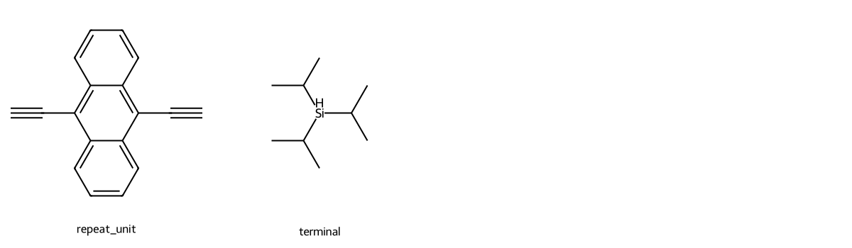
Here are the substructures we’re searching for now:
mols_to_match = []
for sml in smls_to_match.values():
    mol = rotate_90(sml)
    mols_to_match.append(mol)
image = Draw.MolsToGridImage(
    mols=mols_to_match,
    legends=smls_to_match.keys(),
    molsPerRow=4,
    subImgSize=(300, 350),
)
display(image)
df = add_match_counts(
    df=df,
    smls_to_match=smls_to_match,
)
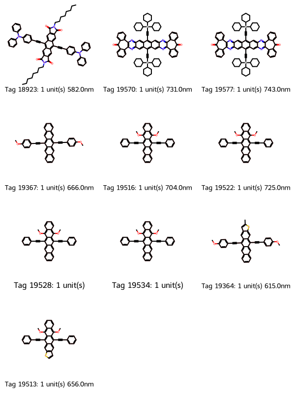
df_to_grid_image(
    df.filter(
        (pl.col("repeat_unit_match_count") > 0) & (pl.col("terminal_match_count") == 2)
    ).sort(pl.col("repeat_unit_match_count"))
)
19 molecules
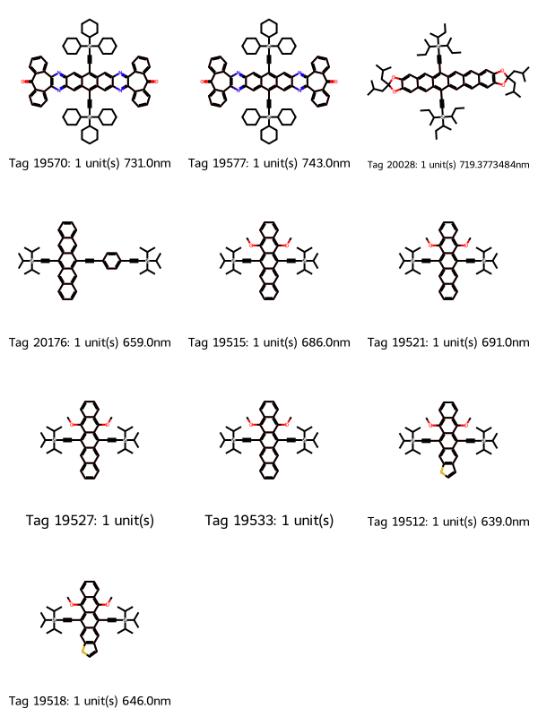
That helps, but we’re getting a lot of fused-ring systems with more than three rings. Let’s exclude those by adding SMILES to match that contain four fused rings, where the fourth ring is either all carbons, or contains two nitrogens. We’ll then filter to molecules whose match count is zero four-fused-ring substructures.
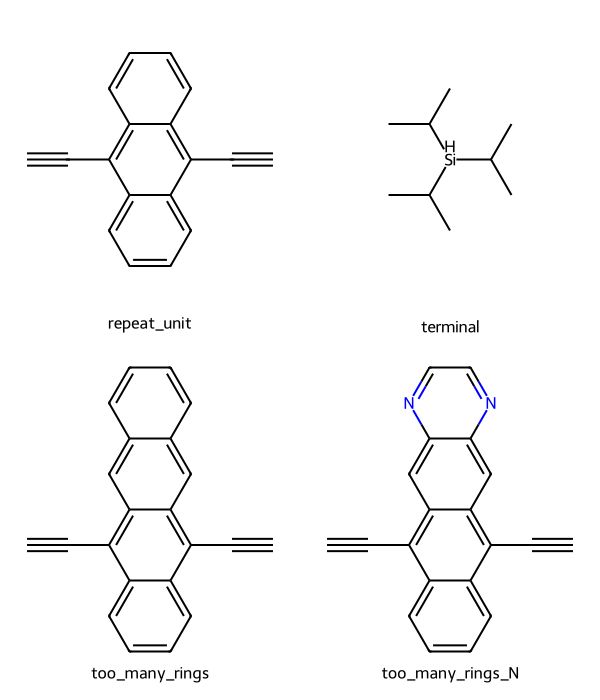
smls_to_match = smls_to_match | {
    # Four benzene rings
    "too_many_rings": "C#CC1=C2C=C3C=CC=CC3=CC2=C(C#C)C2=CC=CC=C12",
    # Four rings: Three benzene and one dinitrogen ring
    "too_many_rings_N": "C#CC1=C2C=C3N=CC=NC3=CC2=C(C#C)C2=CC=CC=C12",
}
Here are all the substructures we’re searching for now, where the first row are substructures we want to include, while the second row is substructures we want to exclude.
mols_to_match = []
for sml in smls_to_match.values():
    mol = rotate_90(sml)
    mols_to_match.append(mol)
image = Draw.MolsToGridImage(
    mols=mols_to_match,
    legends=smls_to_match.keys(),
    molsPerRow=2,
    subImgSize=(300, 350),
)
display(image)
df = add_match_counts(
    df=df,
    smls_to_match=smls_to_match,
)
Next we exclude the four-fused-ring substructures by setting their count to zero.
df_matches = df.filter(
(pl.col("repeat_unit_match_count") > 0)
& (pl.col("terminal_match_count") == 2)
& (pl.col("too_many_rings_match_count") == 0)
& (pl.col("too_many_rings_N_match_count") == 0)
).sort(pl.col("repeat_unit_match_count"))
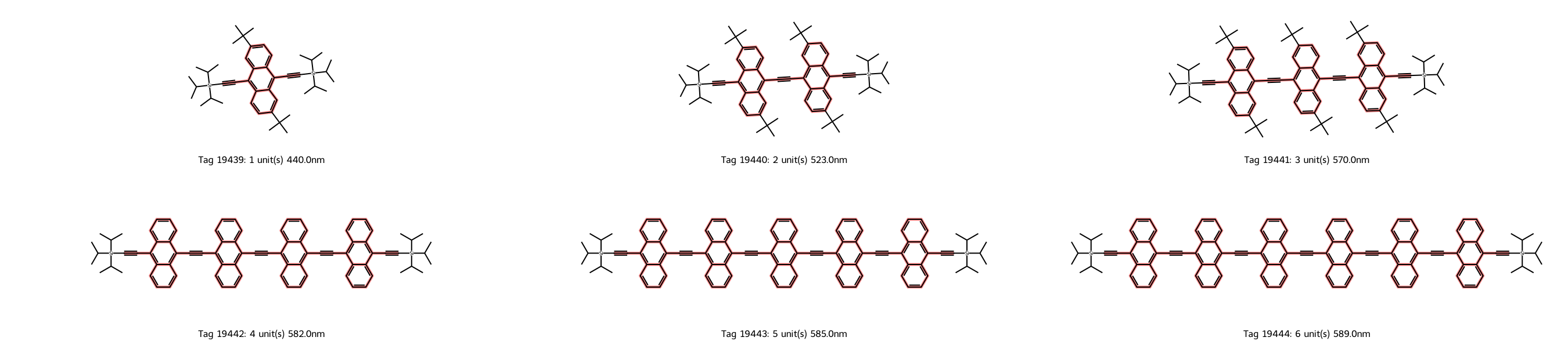
df_to_grid_image(
df_matches,
subImgSize=(900, 300),
molsPerRow=3,
)
6 molecules
df_matches
| Tag | Chromophore | Solvent | Absorption max (nm) | Emission max (nm) | Lifetime (ns) | Quantum yield | log(e/mol-1 dm3 cm-1) | abs FWHM (cm-1) | emi FWHM (cm-1) | abs FWHM (nm) | emi FWHM (nm) | Molecular weight (g mol-1) | Reference | Absorption max (eV) | Emission max (eV) | Stokes shift (eV) | longest_bond_indices | Longest conjugated bond length | repeat_unit_match_count | terminal_match_count | too_many_rings_match_count | too_many_rings_N_match_count |
|---|---|---|---|---|---|---|---|---|---|---|---|---|---|---|---|---|---|---|---|---|---|---|
| i64 | str | str | f64 | f64 | f64 | f64 | f64 | f64 | f64 | f64 | f64 | f64 | str | f64 | f64 | f64 | list[i64] | i64 | i64 | i64 | i64 | i64 |
| 19935 | "CC(C)[Si](C#Cc1c2ccc(C(C)(C)C)… | "Cc1ccccc1" | 440.0 | 461.0 | null | 0.92 | 4.4133 | 2192.4 | 1449.0 | 42.5 | 30.8 | 650.470305 | "10.1021/acs.joc.8b00311" | 2.817771 | 2.689413 | 0.128358 | [4, 5, … 47] | 20 | 1 | 2 | 0 | 0 |
| 19936 | "CC(C)[Si](C#Cc1c2ccc(C(C)(C)C)… | "Cc1ccccc1" | 523.0 | 541.0 | null | 0.02 | 4.694605 | 3158.9 | 1770.3 | 87.0 | 51.9 | 962.658106 | "10.1021/acs.joc.8b00311" | 2.370591 | 2.291718 | 0.078874 | [4, 5, … 74] | 39 | 2 | 2 | 0 | 0 |
| 19937 | "CC(C)[Si](C#Cc1c2ccc(C(C)(C)C)… | "Cc1ccccc1" | 570.0 | 589.0 | null | 0.022 | 4.781037 | 3541.0 | 911.6 | 116.2 | 31.6 | 1274.845907 | "10.1021/acs.joc.8b00311" | 2.175122 | 2.104956 | 0.070165 | [4, 5, … 101] | 58 | 3 | 2 | 0 | 0 |
| 19938 | "CC(C)[Si](C#Cc1c2ccc(C(C)(C)C)… | "Cc1ccccc1" | 582.0 | 609.0 | null | 0.02 | 4.975432 | 3895.7 | 1206.4 | 133.7 | 44.8 | 1587.033707 | "10.1021/acs.joc.8b00311" | 2.130274 | 2.035828 | 0.094446 | [4, 5, … 128] | 77 | 4 | 2 | 0 | 0 |
| 19939 | "CC(C)[Si](C#Cc1c2ccc(C(C)(C)C)… | "Cc1ccccc1" | 585.0 | 623.0 | null | 0.018 | 5.130334 | 3751.8 | 1204.5 | 130.0 | 46.8 | 1899.221508 | "10.1021/acs.joc.8b00311" | 2.119349 | 1.990079 | 0.12927 | [4, 5, … 155] | 96 | 5 | 2 | 0 | 0 |
| 19940 | "CC(C)[Si](C#Cc1c2ccc(C(C)(C)C)… | "Cc1ccccc1" | 589.0 | 629.0 | null | null | 5.178977 | 3681.3 | 1318.7 | 129.2 | 52.3 | 2211.409309 | "10.1021/acs.joc.8b00311" | 2.104956 | 1.971096 | 0.133861 | [4, 5, … 182] | 115 | 6 | 2 | 0 | 0 |
Great! We have just the molecules we want, and the dataset contains all six oligomers with the anthracene repeat unit: n = 1-6.
By the way, those four substructure criteria are sufficient to get just the set of molecules we want from this dataset. If we had a larger dataset, we might have to add more criteria to exclude other molecules.
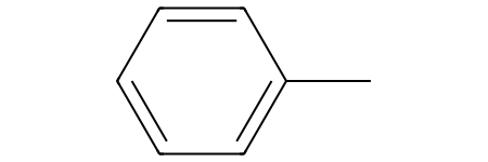
Also, the solvent is toluene in all cases, meaning there are no different solvent effects to consider.
Chem.MolFromSmiles(df_matches[0]["Solvent"].item())
It turns out these molecules all come from one paper, “Synthesis and Electronic Properties of Length-Defined 9,10-Anthrylene−Butadiynylene Oligomers” by Nagaoka et al., DOI 10.1021/acs.joc.8b00311. They actually made this series of molecules for their optical properties: “These oligomers will be attractive as core units in the molecular design of linear π-conjugated compounds for functional dyes and electronic devices.” Their calculated Stokes shift are the same as in our table above.
They also note that the “reaction mixture instantly turned deep purple as a result of the formation of a mixture of oligomers.” This is in agreement with our earlier statement about complimentary colors: Because the n = 1-6 oligomers absorb from 440-589 nm, the complimentary colors will include purple.
As a side note, from examining the dataframe, the photoluminescence quantum yield is 0.92 for n = 1, and about 0.02 for n = 2-5 (a value is not provided for n = 6). Nagaoka et al. attribute this to the fact that “the presence of diacetylene moieties facilitates quenching via nonradiative pathways, as reported for other butadiyne compounds.”
Plot results to check for correlation between color and conjugation chain length
Now that we have a consistent series of molecules, let’s plot their optical properties to check for trends. We’ll use the altair library that provides Polars’ plotting capability.
We start by setting our shape scheme for the absorption, emission, and Stokes shift series.
emission_shape = "circle"
absorption_shape = "triangle"
stokes_shape = "square"
Next we calculate plot ranges based on the data. For all axes, we’ll allow for a slight buffer so our data points aren’t on an edge of the plot.
# Calculate the minimum and maximum y-value in nm across the absorption and emission series
min_y_value_nm = min(
    df_matches["Absorption max (nm)"].min(), df_matches["Emission max (nm)"].min()
)
y_min_nm = min_y_value_nm * 0.95
max_y_value_nm = max(
    df_matches["Absorption max (nm)"].max(), df_matches["Emission max (nm)"].max()
)
y_max_nm = max_y_value_nm * 1.05

# Calculate the minimum and maximum y-value in eV across the absorption and emission series
min_y_value_eV = min(
    df_matches["Absorption max (eV)"].min(), df_matches["Emission max (eV)"].min()
)
y_min_eV = min_y_value_eV * 0.95
max_y_value_eV = max(
    df_matches["Absorption max (eV)"].max(), df_matches["Emission max (eV)"].max()
)
y_max_eV = max_y_value_eV * 1.05

# Calculate the maximum y-value in eV for the Stokes shifts
stokes_y_max = df_matches["Stokes shift (eV)"].max() * 1.1

# Calculate the maximum x-value for all series, based on the maximum repeat unit count
max_repeat_count = df_matches["repeat_unit_match_count"].max() + 0.5
Now we can plot the data. Let’s start with the wavelength units in the source dataset, namely nanometers (nm). We’ll make a scatter plot for the absorption series, then one for the emission series, and layer them on top of each other. To emphasize the color of the light, let’s make each symbol the approximate color of that light, for example 440 nm is violet. For the legend, we’ll make a separate “plot” and concatenate it horizontally with the main plot.
# Order of curves from top to bottom
shapes = [emission_shape, absorption_shape]

# Larger data point size for better visibility
point_size = 150

# Thickness of black outline on data points
stroke_width = 2

# Define a color scale that corresponds to the visible spectrum
color_scale = alt.Scale(
    domain=[380, 700],  # Wavelength range (approximate visible light)
    range=[
        "#8B00FF",  # Violet (~380 nm)
        "#0000FF",  # Blue (~450 nm)
        "#00FF00",  # Green (~520 nm)
        "#FFFF00",  # Yellow (~580 nm)
        "#FF7F00",  # Orange (~600 nm)
        "#FF0000",  # Red (~700 nm)
    ],
)

# Absorption scatter plot with black stroke and fill color based on wavelength
scatter_absorption = (
    alt.Chart(df_matches)
    # Black border with a fill color
    .mark_point(size=point_size, filled=True, stroke="black", strokeWidth=stroke_width)
    .encode(
        x="repeat_unit_match_count",
        y="Absorption max (nm)",
        color=alt.Color(
            "Absorption max (nm)",
            # Fill color corresponds to wavelength
            scale=color_scale,
            title="Wavelength (nm)",
            legend=None,
        ),
        shape=alt.value(absorption_shape),
        tooltip=["repeat_unit_match_count", "Absorption max (nm)"],
    )
    .properties(title="Absorption max")
)

# Emission scatter plot with black stroke and fill color based on wavelength
scatter_emission = (
    alt.Chart(df_matches)
    # Black border with a fill color
    .mark_point(size=point_size, filled=True, stroke="black", strokeWidth=stroke_width)
    .encode(
        x="repeat_unit_match_count",
        y="Emission max (nm)",
        color=alt.Color(
            "Emission max (nm)",
            # Fill color corresponds to wavelength
            scale=color_scale,
            title="Wavelength (nm)",
            legend=None,
        ),
        # Shape for emission
        shape=alt.value(emission_shape),
        tooltip=["repeat_unit_match_count", "Emission max (nm)"],
    )
    .properties(title="Emission max")
)

# Manually create a legend for shapes with the reordered entries (Emission on top, Absorption on bottom)
legend_data = pl.DataFrame(
    {
        "Type": [
            "Emission max (eV)",
            "Absorption max (eV)",
        ],
        # Reordered: Emission first, Absorption second
        "Shape": shapes,
    }
)

legend = (
    alt.Chart(legend_data)
    .mark_point(size=point_size)
    .encode(
        y=alt.Y(
            "Type:N",
            sort=[
                "Emission max (eV)",
                "Absorption max (eV)",
            ],  # Explicit sort order
            axis=alt.Axis(orient="right"),
            title="",
        ),
        shape=alt.Shape(
            "Shape:N",
            scale=alt.Scale(domain=shapes, range=shapes),
            # Disable shape legend
            legend=None,
        ),
        # Keep legend shapes black for distinction
        color=alt.value("black"),
    )
)

# Combine the scatter plots
scatter_combined = (
    alt.layer(scatter_absorption, scatter_emission)
    .properties(title="Optical Properties of Oligomer Series")
    .encode(
        y=alt.Y(
            "Absorption max (nm)",
            scale=alt.Scale(domain=[y_min_nm, y_max_nm]),
            title="Absorption or Emission Max (nm)",
        ),
        x=alt.X(
            "repeat_unit_match_count",
            scale=alt.Scale(domain=[0.5, max_repeat_count]),
            title="Number of Repeat Units",
        ),
    )
    .interactive()
)

# Combine the scatter plot with the legend
final_chart = alt.hconcat(scatter_combined, legend)

# Display the chart
final_chart.show()
For this series with 1-6 repeat units, the absorption (and emission) wavelength maxima indeed show a monotonic increase with increasing number of repeat units, which correlates to the length of the conjugated bond chain. So having a consistent molecular structure demonstrates that increasing the conjugated bond chain length increases the absorption maximum. Nagaoka et al. state this as “The bathochromic shifts [to higher wavelengths] in the UV−vis spectra suggested that the π-conjugation was extended with elongation of the linear chain.” They thus experimentally investigated the question of whether the conjugated bond chain was extended by adding more repeat units, and concluded that it was. This is also expected from their
- X-ray structure of the
n = 3oligomer: “The three anthracene plans are approximately coplanar along the linear molecular axis” - Density Functional Theory (DFT) structure of all six oligomers: “the anthracene groups are coplanar…In these coplanar conformations, the molecular orbitals spread over the acetylene [adjacent carbons joined by a triple bond] and anthracene moieties at the HOMO and LUMO levels”.
If the anthracene groups were not coplanar, the p orbitals on the acetylene and anthracene units would not be pointing in the same direction, potentially disrupting the conjugated bond chain. The RDKit method bond.GetIsConjugated() examines the molecular graph (with atoms as nodes and bonds as edges), which does not consider things like bond angles, so the experimental data more conclusively demonstrate that the conjugated bond chain length is increased with more repeat units.
Nagaoka et al. note “These results suggest that diacetylene linkers effectively mediate electronic communication between aromatic units”.
As we discussed earlier, for comparisons such as the Stokes shift, it’s better to plot in terms of energy. Let’s do that and add the Stokes shift on the same x-axis, but below the main plot.
# Order of curves from top to bottom
shapes = [absorption_shape, emission_shape, stokes_shape]

# Larger data point size for better visibility
point_size = 100

# First scatter plot for "Absorption max (eV)" and "Emission max (eV)" (upper part of the y-axis)
scatter_absorption = (
    alt.Chart(df_matches)
    .mark_point(size=point_size)
    .encode(
        x="repeat_unit_match_count",
        y=alt.Y("Absorption max (eV)", scale=alt.Scale(domain=[y_min_eV, y_max_eV])),
        color=alt.value("black"),
        shape=alt.value(absorption_shape),
        tooltip=["repeat_unit_match_count", "Absorption max (eV)"],
    )
)

scatter_emission = (
    alt.Chart(df_matches)
    .mark_point(size=point_size)
    .encode(
        x="repeat_unit_match_count",
        y=alt.Y(
            "Emission max (eV)", scale=alt.Scale(domain=[y_min_eV, y_max_eV])
        ),  # Same y-axis range as absorption
        color=alt.value("black"),
        shape=alt.value(emission_shape),
        tooltip=["repeat_unit_match_count", "Emission max (eV)"],
    )
)

# Second scatter plot for "Stokes shift (eV)" (lower part of the y-axis)
scatter_stokes = (
    alt.Chart(df_matches)
    .mark_point(size=point_size)
    .encode(
        x="repeat_unit_match_count",
        y=alt.Y(
            "Stokes shift (eV)",
            # Stokes shift on a different y-axis range
            scale=alt.Scale(
                domain=[0, stokes_y_max],
            ),
        ),
        color=alt.value("black"),
        shape=alt.value(stokes_shape),
        tooltip=["repeat_unit_match_count", "Stokes shift (eV)"],
    )
)

# Update legend data with shape information
legend_data = pl.DataFrame(
    {
        "Type": ["Absorption max (eV)", "Emission max (eV)", "Stokes shift (eV)"],
        "Shape": shapes,
    }
)

# Manual legend with explicit sort order
legend = (
    alt.Chart(legend_data)
    .mark_point(size=100)
    .encode(
        y=alt.Y(
            "Type:N",
            # Explicit sort order
            sort=[
                "Absorption max (eV)",
                "Emission max (eV)",
                "Stokes shift (eV)",
            ],
            axis=alt.Axis(orient="right", title=None),
        ),
        color=alt.value("black"),
        shape=alt.Shape(
            # Map the Shape column to the shapes in the legend
            "Shape:N",
            scale=alt.Scale(
                domain=shapes,
                range=shapes,
            ),
            # Disable shape legend
            legend=None,
        ),
    )
)

# Layer the absorption and emission scatter plots
upper_chart = alt.layer(scatter_absorption, scatter_emission).encode(
    y=alt.Y(
        "Absorption max (eV)",
        scale=alt.Scale(domain=[y_min_eV, y_max_eV]),
        title="Absorption or emission maximum (eV)",
    ),
    x=alt.X(
        "repeat_unit_match_count",
        scale=alt.Scale(domain=[0.5, max_repeat_count]),
        title=None,
        axis=alt.Axis(labels=False, tickSize=0),
    ),
)

# Create the Stokes shift scatter plot
lower_chart = scatter_stokes.encode(
    y=alt.Y(
        "Stokes shift (eV)",
        scale=alt.Scale(domain=[0, stokes_y_max]),
        title="Stokes shift (eV)",
    ),
    x=alt.X(
        "repeat_unit_match_count",
        scale=alt.Scale(domain=[0.5, max_repeat_count]),
        title="Number of repeat units",
    ),
)

# Combine the two charts vertically with some padding to simulate a break
combined_chart = alt.vconcat(
    upper_chart.properties(height=300), lower_chart.properties(height=100), spacing=10
).resolve_scale(x="shared")

# Display the combined chart with the legend
layered_chart = alt.hconcat(combined_chart, legend)

layered_chart.show()
The y-axis makes it easier to compare energy values both between and within molecules. This plot agrees with Nagaoka et al’s statement that “HOMO—LUMO gaps [absorption maxima, in eV] decrease with an increasing chain length”.
The Stokes shift is relatively constant, ranging between 0.7 and 0.14 eV, despite the absorption maximum decreasing by ~0.7 eV from n = 1 to n = 6, because the emission maximum follows the same trend. The Stokes shift does show a trend, decreasing from n = 1 until n = 3, then increasing up to n = 6, which may be due to conflicting factors.
Conclusions
By finding a series of molecules with a consistent structure, and from 1-6 repeat units, we found that absorption maximum increases (from the ultraviolet to the visible) as the length of the conjugated bond chain increases, as predicted by molecular orbital theory. This effect helps explain why some organic molecules are colored.
By changing the conjugated bond chain length, chemists can tune the optical properties of absorption and emission wavelength to make useful devices. It’s important to verify experimentally that the absorption wavelength maximum does in fact increase, indicating that the electrons can spread over more bonds, when the chain length (as determined by cheminformatics) is increased.
Revisions
- 2024-10-20 Revised to display bond indices using RDKit’s
addBondIndices. - 2024-10-24 Used revision 3 of Experimental database of optical properties of organic compounds, which Sungnam Park updated to correct molecular structures after I shared discrepancies in the structures of the
n = 4-6oligomers compared to the paper of Nagaoka et al.